Time Based Profile (Trapezoidal Acceleration)
| Language: | English • 中文(简体) |
|---|
Contents
General Introduction
This document describes the time-based trapezoidal acceleration motion profiler in the softMC. In order to understand the features of this profiler, we first describe the sine acceleration profiler implementation.
Both profilers are basically state machines that change their states during path generation and based on each state use different formulas to compute the profiler output (position, velocity, acceleration). These states are: acceleration increase, acceleration saturation, acceleration decrease, zero acceleration.Some states can be repeated during motion (e.g., an acceleration state, followed by a deceleration state) and some can be completely omitted (e.g., zero acceleration in short motions).
The main difference between these two profilers is the state-selection algorithm i.e., condition on which the system switches from one state to another. The current implementation (firmware since Version 4.5.25) is dominantly velocity based. This means that the current velocity value is the main criteria for the sine acceleration profiler to switch to another state or not. However, the velocity value is not enough, so additional internal variables are also being used: phase angle, target distance, profiler state.


The trapezoidal acceleration profiler (since Version 4.5.25) has a state-change condition based only on one variable – the current time. The off-line pre-calculation (which is common to both profilers) pre-calculates switching times for each state and this gives a simple condition when the states should be changed.
Such an approach provides some benefits over the velocity based profiler. One of these is the introduction of safe SP blending feature.
| Time Based Profiler | Velocity Based Profiler | |
| RTK load | Braking distance checked in each sample. | Braking distance checked in each sample. |
| Time discretization – sample falls between different phases | None, as (p,v,a) values are computed on the current time value only | We need to separately compute each of the phases and then to subtract. |
| Easy online changes of the target point | Whole pre-computation needs to be repeated | As braking distance is always checked, it goes relatively painless. |
| Time driven events (i.e., to define an event on a specific time instance (before reaching the target point)) | A simple built-in feature | Very inconvenient to implement, as we actually have no idea about the total execution time of the movement |
| Prediction of the total execution time (e.g., in SP blending, preventing a third motion to enter before the second is finished) | A simple built-in feature | Very inconvenient to implement, as we actually have no idea about the total execution time of the movement |
Implementation Specifics
Language interface.
Originally the system supported only two types of motion profiles: sine acceleration(SA) and trapezoidal velocity (TV). The user selected a motion profile by defining the smooth factor: 0 – TV, everything else is a SA profile. This is very intuitive, as TV is the least smoothest profile that the user can choose (kind of singular profile). But, this is very inconvenient for defining other profile types. Therefore a new property was introduced:
<ELEMENT>.PROFILERTYPE
Profiler Specific

Currently, the only implemented time-based profiler is the trapezoidal acceleration profiler. The time-based profiler gives a smooth velocity and position profile (“S”-curve). Compared to the sine-acceleration profile, this profile has a reduced jerk value for the same amount of acceleration and has one more jerk discontinuity point in the acceleration profile. However, considering that the jerk value is also about three times lower (3.14 times), it can be assumed that the two profiles are basically the same. The transformation of TA into TV is done by reducing acceleration increase time to be shorter then the motion sample, contrary to the SA profile, where this transformation is sometimes done silently (acceleration time less than 5 samples). In this profile type the velocity smoothness will be assured by having J/A > T.

Side effects:
The trapezoidal acceleration profile (TA) is not able of having a non-zero initial and/or final velocity. This constraint causes the following limitations on use of ProfileType=2:
- The execution of VORD change is postponed to the first motion entered after its change, i.e., there is no on-line change of velocity command.
- Motion with StartType immediate or fast-immediate is not allowed with this profile.
- In SP-Blending mode, a feature is available for preventing entering a third movement before the second one is complete.
- The TA profiler allows introducing time-events prior to motion end.
- Concatenation (Vfinal ≠ 0) – not possible as this type of profiler does not accept non-zero initial and/or final velocities.
- BlendingMethod = 1 (Continuous Path) is not be functional with (PrfType = 2). In this case blending is done in profile-following mode where only one motion executes profile and the other just follows it:
- BlendingMethod = 2 (Super-Position) is fully operational.
- BlendingMethod = 3 (AI) is fully functional and independent from selected profile type.
New blending properties
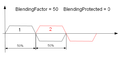
Illustration 4: BlendingFactor = 50 BlendProtected = 0
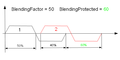
Illustration 5: BlendingFactor = 50 BlendProtected = 60
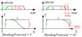
Illustration 6: BlendProtected = 40 and BlendProtected = 0
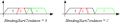
Illustration 7: BlendingStartCondition=0 and BlendingStartCondition=1


Coding Issues
Both the time-based and velocity-based profilers have three different functional parts:
- Pre-Computation part, where the given user parameters of velocity, acceleration and jerk are transformed into actual operational values.
- Real-time executioner that is called each sampling period and produces the next (position, velocity, acceleration) triple.
- Inverse profiler function, a routine that computes internal profiler parameter based on given position inside profiler path. In velocity based profile this function is non-trivial, in time based profile this function is much simpler and is in the form of t = Profiler-1(p). This ability is crucial in implementing BlendProtected feature of the SP blending.

See Also
--Mirko 08:22, 20 December 2010 (CET)