AXY:Pre-Computation Modes

Discussions

	NOTE
	Goal: Achieve a constant upper limit of joint limit violations during Cartesian motion with acceptable effort (implementation and run-time load) (Fritz, Artur, Raul, Torsten, Mirko during Manz visit November 2009)

Status

• Some models have rough mechanisms (Inertia Threshold)
• Assumptions aren't very precise
• Singularities are not treated at all

Motivation

• Internal complains in SCARA and PUMA systems.
• Expectations of users of the upcoming SuperDrive-System not to see the same
• Exceptions resulting from joint limit violations
• First step: In robot groups throwing a note in case of joint limit exceeded (velocity and acceleration in case of SP, CT and Cartesian trajectory)
• In single axis motion the slaved axis throws an error (DIFFERS from group)

Modes

Fast: Current mode of pre-computation considering some points on the path with prediction of vel, acc at these points and consider the joint limits.

Zero: Alternative mode where no joint limits are checked

Optimum: Iterative pre-processing along the path

Self-tuning: Motions adopted during run-time by observation of percentage and store look-up table with spatial and velocity dimensions (default is low, going to limit is learned). Can be used during start-up phase of a machine (no change during operation with customer)

Pre-calculated look-up mode: Similar to SysMot.lib; the look-up is not self-learned, but user-defined

Handle singularities in Cartesian trajectory motion

• Slow down the motion to the value needed near the singularity. (if constant velocity is required)
• Cut the motion into pieces where near singularity lower accelerations and velocities can be used. (if no constant velocity is required)
• Similar to the non-constant velocity mode above, cut the motion into pieces and switch
• to joint motion in an epsilon around the singularity where the joint limits are exceeded.
  Torsten: Stäubli claims to compute the mostsingular-point in cartesian space during pre-planning and then act accordingly.

Additional

Have a callback function which returns a reduction factors for velocity, acceleration and deceleration based on internal considerations (as strut/rod/joint forces) not existing in the general softMC motion model. IDM automatically calculates the acceleration reduction for robot models according to TMAX (which is not used today).

Payload introduced to the model makes changes to joint limits not necessary anymore.

	NOTE
	Checking of AMAX gets kind of obsolete (or just additional user limitation)

Action items

• Extend IDM for callback function in 4.5.x

• Add precalculation mode “Zero”

• Add “Self-tuning” and “pre-calculated” mode

• Add precalculation mode “Optimum”

• Add SCARA model to IDM

• Replace AF Payload mechanism by IDM Payload and TMAX limit

• Add PUMA model to IDM

• Trajectory motion (non constant velocity, partial joint)

Introduction

Each movement command is executed in two phases, first the pre-computation phase and the second phase where the movement iterations of the position and velocity of each axis are computed every sample period. The pre-computation is done after interpreter processes the motion command (MOVE, JOG, MOVES, ...) and sends message to the Motion Manager Task which executes the actual pre-computation. During the pre-computation, operational velocity acceleration and jerk values of the movements are computed. This is done considering different sets of limitations:

• System Limitations: values of vrate,arate,drate and vord
• Group limitations: values of vmax,amax,dmax,jmax (vmtran,amtran,jmtran/vmrot,amrot,jmrot)
• Joint Limitations: values of vmax, amax, jmax, tmax of each joint involved in the motion reached during specific motion
• Profile Limitations: mutual relation of L,V,A,D,J

Definitions

L – length

V - velocity

A - acceleration

D - deceleration

J – jerk

$q_{i}$- joint coordinate, i-th joint

${{\dot {q}}_{\mathit {max}}}_{i}$- max velocity of joint i

${q}_{\mathit {start}}$- joint coordinate of start point

${P}_{\mathit {start}}$- cartesian coordinate of the start point

${q}_{\mathit {target}}$ - joint coordinate of target point

${P}_{\mathit {target}}$- cartesian coordinate of the target point

${P}_{0}$- cartesian coordinate of the start point

${P}_{1}$- cartesian coordinate of the target point

MMT Motion Manager Task

RTK Real Time Kernel

MCO Motion Category Object

Motivation

Ideally values of joint (motor) torque, acceleration, velocity should not exceed maximal motor values and in case of fast-as-possible movements they should reach them (but not exceed).

• If these values are exceeded we can get drive errors (PCMDVCDM error) or the position following error can develop (pe > pemax).
• Typically (in today's implementation) the v&a values are not extremely exceeded so the following error is not building up to the value that it can be noticed, but the PCMDVCDM drive error do react causing application to stop.
• Additionally, the built-in position limit protection algorithm can trigger-in (as value of dmax is smaller then actual value and causes longer stopping path) and “max/min position limit reached” error can cause application to stop.
• In cases of sensitive mechanics (DELTA) such high acc/jerk values can even lead to robot disassembling.
• If the motion is over-compensated all the above cases will not occur but then the overall application's cycle time will be increased.
  

Current Implementation

MOVE (joint interpolation)

This is the most straight-forward case. As the motion of individual joints is in pure proportion to the group motion the maximal values of each joint can be exactly computed. Shortly in case of joint-interpolated motion we are in ideal case.

MOVES (Cartesian straight line)

Global Joint Velocity Limitation

using given cruise velocity as average velocity we obtain an average total movement time which again is used to calculate the average joint velocity. If this is bigger then max joint velocity the cartesian cruise velocity will be reduced.

Failed to parse (unknown function "\begin{gathered}"): {\displaystyle \begin{gathered}T=\frac{L}{V_{\mathit{cruise}}}\\V_{\mathit{joint}}=\frac{\left|{\left|{\boldsubformula{q}_{\mathit{target}}-\boldsubformula{q}_{\mathit{start}}}\right|}\right|}{T}\\K=\mathit{max}(\frac{(\boldsubformula{q}_{\mathit{target}}-\boldsubformula{q}_{\mathit{start}})_{i}}{\left|{\left|{\boldsubformula{q}_{\mathit{target}}-\boldsubformula{q}_{\mathit{start}}}\right|}\right|})\cdot {\frac{V_{\mathit{joint}}}{{{\dot{q}}_{\mathit{max}}}_{i}}}\end{gathered} }

Axes Motion Limitations

Selected Cartesian points are tested according to following algorithm:

Inverse Dynamic & Kinematics on each point using selected acceleration and velocity is computed and values of joint velocity, acceleration and torque are obtained. These are checked against max joint values ad the overall max reduction rate is used to reduce the given cruise velocity:

Failed to parse (unknown function "\begin{gathered}"): {\displaystyle \begin{gathered}(\boldsubformula{q},\dot{\boldsubformula{q}},\ddot{\boldsubformula{q}},\boldsubformula{\tau })=\mathit{IDM}(P,V,A)\\K_{V}=\mathit{max}\frac{\dot{\boldsubformula{{q_{i}}}}}{\mathit{vmax}_{i}}\ \ \text{velocity factor}\\K_{A}=\mathit{max}\frac{\ddot{\boldsubformula{q}}_{i}}{\mathit{amax}_{i}}\ \ \text{acceleration factor}\\K_{T}=\mathit{max}\frac{\boldsubformula{\tau }_{i}}{\mathit{tmax}_{i}}\ \ \text{torque factor}\\K=\mathit{max}(K_{V},K_{A},K_{T})\end{gathered}}

where: ${\mathit {IDM}}(P,V,A)$ is the Inverse Dynamic Model of the system, Failed to parse (unknown function "\boldsubformula"): {\displaystyle \boldsubformula{q}} is vector of joint coordinates, Failed to parse (unknown function "\boldsubformula"): {\displaystyle \boldsubformula{\tau }} is vector of joint force/torques and P is Cartesian position vector.

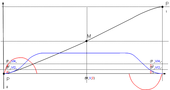
Points checked (current implementation)

Path middle point $(P_{M},V_{\mathit {cruise}},0)$(in SCARA instead of the middle point we use the point closest to X=0 & Y=0).

	NOTE
	Note the assumption of using cruise velocity(?) with zero acceleration(?) at the given point.

This step reduced the cruise velocity: $V_{\mathit {cruise}}^{o}={\frac {1}{K}}V_{\mathit {cruise}}$

Four test points with their associated velocities and accelerations are checked:

• initial point: $(P_{0,}{\frac {1}{2}}V_{\mathit {cruise}},A)\ (P_{0,}{\frac {1}{4}}V_{\mathit {cruise}},A)$ (assumption is having max acceleration at motion start)
• final point:$(P_{1,}{\frac {1}{2}}V_{\mathit {cruise}},-D)\ (P_{1,}{\frac {1}{4}}V_{\mathit {cruise}},-D)$ (assumption is having max deceleration at motion end)

where $(P_{0}\ \ P_{1})$ are initial and final points of the move.

This step reduces acceleration and deceleration of the move as:

$A^{o}={\frac {1}{{\mathit {max}}(K_{A},K_{T})}}\cdot A$ and $D^{o}={\frac {1}{{\mathit {max}}(K_{D},K_{T})}}\cdot D$

	NOTE
	Notice the influence of torque to acceleration only (no velocity). This is clearly not true but is taken s another approximation of the real relationships.

	NOTE
	Above formulas present the general ideas only the small issues like zero division and limiting max values in singular point cases and limiting max values above 1 ware omitted for clarity reasons only.

(M,V,0)(P₁,V/2,-D)(P₁,V/4,-D)(P₀,V/2,A)(P₀,V/4,A)MP₁P₀

Drawing 1: Five test points that are used for checking

CIRCLE (Cartesian)

Basically same limitation are used as in straight line case except the units are angular. Also additionally evenly distributed points on the circle arc are checked for reachability.

ADVANCED INTERPOLATION

Only global joint limitation is done (see 4.2.1 Global Joint Velocity Limitation ) TBD

Blending

Continuous Path (CP)

Limitation is done per each motion and in context of continuous blending.

Superposition (SP)

Limitation is done per each motion involved but not as combination therefore overshoots can occur.

Summary of current implementation

The currently implemented limitation algorithm uses several simplifications that can increase the error of estimating maximum motion values more or less:

• Using only several pre-selected points (initial, middle, final) although the real maximum can occur somewhere else.
• Using arbitrary acceleration and velocity values at these points.
• Assuming the torque is influenced by the acceleration only.
• Assuming linear relationship between cartesian and joint max values.

Theoretic solution

The theoretical points of maximum joint velocity, acceleration and torque are:

Failed to parse (unknown function "\begin{gathered}"): {\displaystyle \begin{gathered}\boldsubformula{\dot{q}}_{v}=\boldsubformula{J}(\boldsubformula{q}_{v})\cdot \dot{\boldsubformula{p}}(t_{v})\\\boldsubformula{\ddot{q}}_{a}=\boldsubformula{J}(\boldsubformula{q}_{a})\cdot \ddot{\boldsubformula{p}}(t_{a})+\delta \boldsubformula{J}(\boldsubformula{q}_{a},\boldsubformula{\dot{q}}_{a})\cdot \dot{\boldsubformula{p}}(t_{a})\\\boldsubformula{\tau }_{T}=H(\boldsubformula{q}_{T})\ddot{\boldsubformula{q}}_{T}+\boldsubformula{\dot{q}}_{T}\cdot C(\boldsubformula{q}_{T})\cdot \boldsubformula{\dot{q}}_{T}+G(\boldsubformula{q}_{T})\end{gathered}}

where

J – robot Jacobian matrix

H – inertia matrix

C – centrifugal and Coriolis components

G – gravity components

q – joint coordinates vector

p – cartesian coordinates vector

τ - joint torques vector

Or in case when the IDM system feature is used:

Failed to parse (unknown function "\begin{gathered}"): {\displaystyle \begin{gathered}\dot{\boldsubformula{q}}_{v}=\mathit{IDM}_{v}(\boldsubformula{p}(t_{v}),\boldsubformula{\dot{p}}(t_{v}),\boldsubformula{\ddot{p}}(t_{v}))\\\ddot{\boldsubformula{q}}_{a}=\mathit{IDM}_{A}(\boldsubformula{p}(t_{a}),\boldsubformula{\dot{p}}(t_{a}),\boldsubformula{\ddot{p}}(t_{a}))\\\boldsubformula{\tau }_{T}=\mathit{IDM}_{T}(\boldsubformula{p}(t_{t}),\boldsubformula{\dot{p}}(t_{t}),\boldsubformula{\ddot{p}}(t_{t}))\end{gathered} }

assuming we know where the max values are reached (e.g know the values of: $(t_{v},t_{a},t_{T})$) it is difficult to find new values of velocity and acceleration. For example if we reduce cartesian velocity proportionally the points of max acceleration $t_{a}$ will clearly move! Notice the third formula, dynamic model of open-chain robots. Here we see that torque is function of joint position and it's both derivatives Failed to parse (unknown function "\boldsubformula"): {\displaystyle (\boldsubformula{q}_{T},\dot{\boldsubformula{q}}_{T},\ddot{\boldsubformula{q}}_{T})} . Basically we should reduce acceleration, but it is not clear at all if we should reduce or increase the velocity as the sign of Coriolis component Failed to parse (unknown function "\boldsubformula"): {\displaystyle C(\boldsubformula{q}_{T})} can differ! What about gravity component Failed to parse (unknown function "\boldsubformula"): {\displaystyle G(\boldsubformula{q}_{T})} – if it is small enough it can be offset-ed from the torque but if not we do not have a solution. Doing all this the max torque point will change, so it is an iterative process!

	NOTE
	Only the first formula is relatively simple, here we have: Failed to parse (unknown function "\boldsubformula"): {\displaystyle \dot{\boldsubformula{p}}(t_{v})=\boldsubformula{J}^{-1}(\boldsubformula{q}_{v})\cdot \boldsubformula{\dot{q}}_{v}} which does not affect $t_{V}$.

	NOTE
	Once these limitations checks are done, the motion parameters are adjusted in the Profiler Limitation calculations again, so everything needs to be re-computed.

	NOTE
	And all this assuming no non-zero initial and/or final velocity and/or robot singular points!

	NOTE
	Note that the above theory says nothing about the jerk (third derivatives) values!

Adding Pre-Computations Modes

In order to enable user to fine tune the motion the PreComputationMode nodal parameter will be added.

<element>.PreComputationMode

Value 0: “None” The whole joint limitation algorithm will be skipped, profiler is generated using motion parameters directly given by the user only limited by profile limitations. Attention! Such mode can be very dangerous as it can lead to extremely fast motions with no regard to actual joint limits.

Value 1: “Realistic” (default) Same as the current implementation.

Value 2: “Optimum”. Iterative pre-processing along the path. Can take long time and depending on the CPU power and motions that are given can dramatically increase the application cycle time.

Value 3:“Self Tuning”. Adaptation process of multiple motion runs. Each motion is stored in a mulch-dimensional table with it's last executed parameters and achievable max joint values. Initially a very conservative approach is taken and as motions are repeated the motion parameters are corrected automatically by the results of executed tries. Needs sophisticated memory handling and table building method. Motions should be somehow sorted according its initial and final position. The robot space should be divided in smaller segments and motions should be sub-categorized accordingly.

Value 4:“user given”. Specific user-written call back functions will be inserted into pre-calculation process. Similar to the current implementation of SysMot.Lib. Function will compute velocity, acceleration, deceleration and jerk reduction factors based on given initial and final position of the movement based on joint max values.

Internal Forces Limitation

Separate call-back function that will compute velocity, acceleration, deceleration and jerk reduction factors based on given initial and final position of the movement based on internal (strut/rod) forces. This function is an additional callback function provided by the user and is independent from the PreComputationMode value set.

Input arguments:

• $P_{0},P_{1}$ initial and final Cartesian points of the motion.
• Failed to parse (unknown function "\boldsubformula"): {\displaystyle \boldsubformula{v}_{c}} vector of cruise velocity
• Failed to parse (unknown function "\boldsubformula"): {\displaystyle \boldsubformula{a}\ ,\ \boldsubformula{J}_{a}} max acceleration & max jerk acceleration vector vectors
• Failed to parse (unknown function "\boldsubformula"): {\displaystyle \boldsubformula{d}\ ,\ \boldsubformula{J}_{d}} max deceleration vector & max jerk declaration vector vectors
  

Output arguments:

• $v_{\text{red}},a_{\text{red}},d_{\text{red}},{\mathit {ja}}_{\text{red}},{\mathit {jd}}_{\text{red}}$reduction factors (percentages). Values that should multiply velocity, acceleration,d deceleration and jerk values in order not to exceed the internal mechanic forces.

Self-Tuning Pre-Computation Algorithm

Activation

This mode is activated by setting the PreComputationMode parameter to 3.

Limitations

The proposed algorithm will be simplified to position only, rotation dominant movements will be not treated by this algorithm.

General Algorithm Description

The self tuning is done in several phases:

• The robot working space will be divided in smaller segments and motions will be categorized according to the pairs of initial and final points.
• The very first motion is started with a set of very conservative parameters.
• During the motion execution a real-time agent function is determining the motion coefficients: $K_{v}^{p}={\mathit {max}}_{i}{\frac {\mathit {Vcmd}}{\mathit {Vmax}}}\ \ K_{a}^{p}={\mathit {max}}_{i}{\frac {\mathit {Acmd}}{\mathit {Amax}}}\ \ K_{T}^{p}={\mathit {max}}_{i}{\frac {\mathit {Tcmd}}{\mathit {Tmax}}}$ where i goes through all axes indexes and p for all motion phases (= isMoving flag).
• At the motion end these coefficients are stored in relation to the movement.
• Next time a similar movement is executed the K parameters are taken and used as additional reduction/multiplication values.

Real-time agent

During motion execution, in the level of the real-time profile generation K-factors will be determined and the motion end placed in a special placer for the next-movement tuning.

Motion categorization and search algorithm

Each movement is categorized according to its initial and final position. A motion category will keep the K factors and the movement parameters (A,D,V)

A	max(Ka,Kt)		D	max(Kd,Kt)		V	Kv
a0	K0		d0	K0		v0	K0
a1	K1		d1	K1		v1	K1
a2	K2		d2	K2		v2	K2
...	....		...	....		...	....
An	Kn		dn	Kn		vn	Kn

Table 1: K-factor table

Where n – is the fixed length size of the table column and values of A, D, V are updated always as monotonically increasing series of values with the smallest value indexed by 0 and the largest value indexed by n.

Filling the K-factor table

The K-factor table is filed by the result of the RTK-agent, each K factor depending from the phase it is detected will be inserted in relevant place of the K-factor table.

In the RTK, each time one of the values is exceeded the relevant K ratio is recorded and the current movement phase is stored (acceleration, cruise, deceleration). Always the max value is stored. At the end of motion a following table is filled (RTK-agent table):

isMoving	Ka	Kd	Kv	Kt	phase	values
1	-	-	-	-	acceleration	(v,a)
2	-	-	-	-	cruise	v
3	-	-	-	-	deceleration	(v,d)

Table 2: RTK-agent table. These values are for specific a,d and v values

At the end of motion the RTK sends a message (especially added for this purpose) to the Motion Manager Task to include this table. The Motion Manager Task finds the corresponding MCO in the data structure and updates the K-factor table. RTK-agent tables will be kept in a ring buffer and independently filled from the RTK and cleared for MM task. An overloading of the ring buffer can not occur as the tables are created and consumed by the same instance (MM task). There could be not more then 3 itmes difference due to blending and velocity-override features.

Data Structure

TYPE '''par''' OF: 
'''acc,vel, Ka,Kd,Kv,Kt''' OF DOUBLETYPE 
'''rtk-agent-table '''OF:acceleration OF par;
cruise OF par;
deceleration OF par;
status: IN-USE, FILLED,EMPTY 
start // cartesian point
target // cartesian point

Updating K-table

The K-factor table is then updated by the following algorithm:

For each column of K-table we do:

• If the column is not filled yet, then just add a row at an appropriate place (keeping the monotonously increasing series).
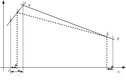
• In case value x is outside the [[Image:]]array or in case it is too close to some of existing values ([[Image:]]) the average value with the closest [[Image:]] is taken and updated into K-table.
• If all columns are filed then find the rows i, i+1 such that new value is in between them and replace the according:
  

Failed to parse (unknown function "\begin{gathered}"): {\displaystyle \begin{gathered}x_{i}<\boldsubformula{x}<x_{i+1}\\w_{i}=\frac{\boldsubformula{x}-x_{i}}{x_{i+1}-x_{i}}\\w_{i+1}=\frac{x_{i+1}-\boldsubformula{x}}{x_{i+1}-x_{i}}\\w_{i}+w_{i+1}=1\\w=\mathit{min}\frac{(w_{i},w_{i+1})}{2}\\{\hat{x}}_{i}=x_{i}+w\cdot (x_{i+1}-x_{i})\\{\hat{y}}_{i}=y_{i}+w\cdot (\boldsubformula{y}-y_{i})\\{}\\{\hat{x}}_{i+1}=x_{i+1}-w\cdot (x_{i+1}-x_{i})\\{\hat{y}}_{i+1}=y_{i+1}-w\cdot (y_{i+1}-\boldsubformula{y})\end{gathered} }

where x is one of (a,d or v) value of K-factor table and y is one of the appropriate K factor.

Data Structure

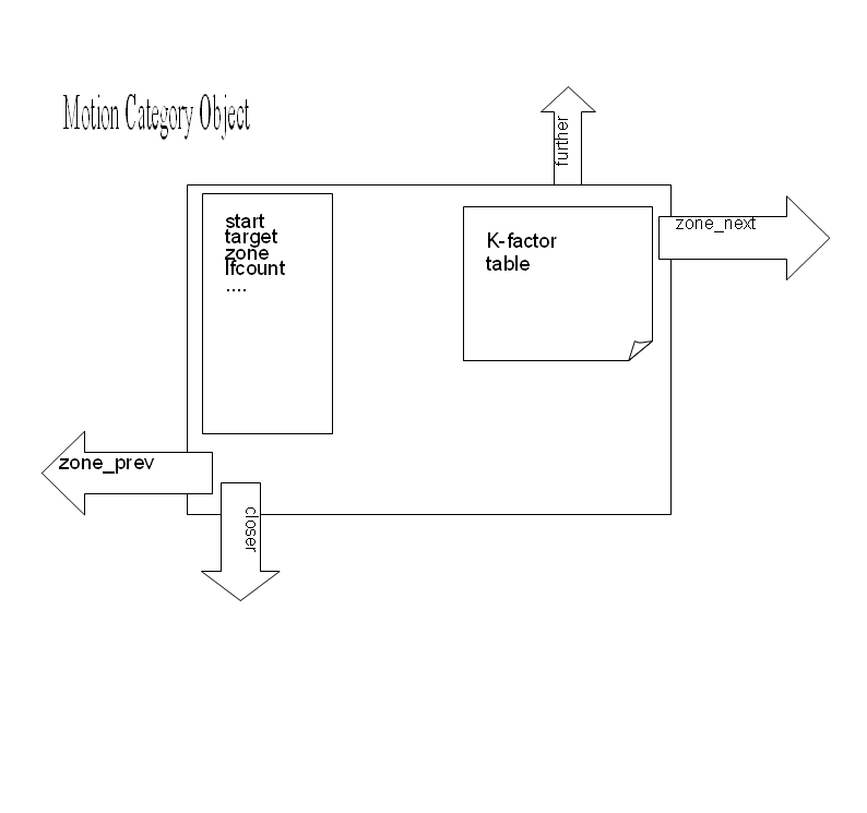
Organizing 3D data is extremely complex tasks. Therefore we will use a simplified model for keeping the measurement results (K-factors). The movement will be stored as a linked structure of objects (Motion Category Object, further: MCO):

K-factortablestarttargetzonelfcount....zone_prevMotion Category Object

where:

• closer, further, zone_next and zone_prev are pointers to the same motion category object.
• start & target are start and target points of the movement.
• zone – zone value of this MCO (see below).
• lfcount – leaf counter, number of elements in the leaf (see below).
  

To each motion category object has a zone weight assigned to it for better sorting, the zone is calculated as:

$z={\mathit {Zone}}(A)=\left|\left|{A_{\mathit {start}}}\right|\right|+\left|\left|{A_{\mathit {target}}}\right|\right|+\left|\left|{A_{\mathit {start}}-A_{\mathit {target}}}\right|\right|$

Additionally we define an auxiliary metric function as:

$d={\mathit {dist}}(A,B)=\left|\left|{A_{\mathit {start}}-B_{\mathit {start}}}\right|\right|+\left|\left|{A_{\mathit {target}}-B_{\mathit {target}}}\right|\right|$

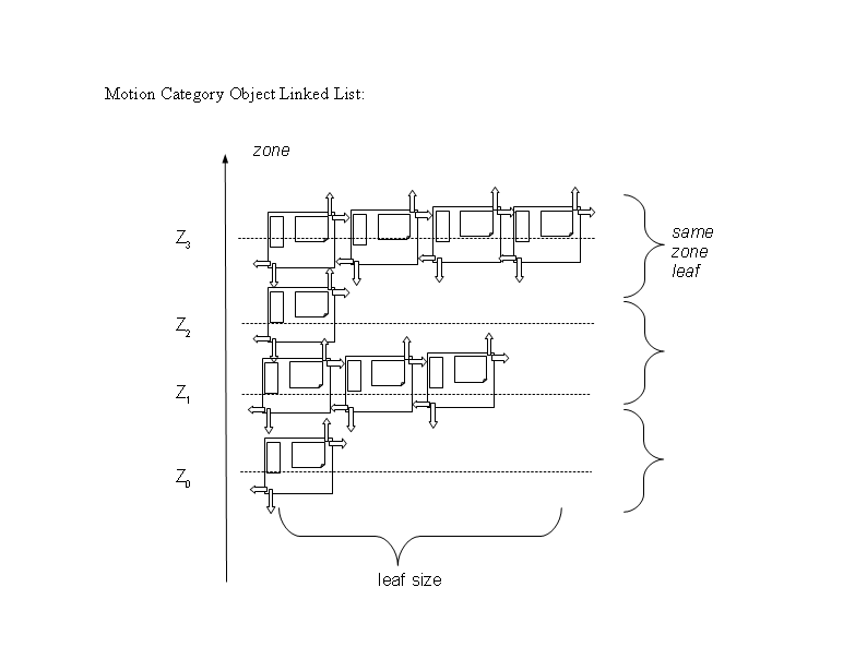
Motion Category Objects are organized in a double -linked list for discrete zone leafs:

Z0Z1Z2Z3zone'same zone leafleaf sizeMotion Category Object Linked List:

where $\Delta Z=Z_{i-1}-Z_{i}$ a user parameter. Leafs of same zones are unsorted single-linked lists of motion category objects. New objects are inserted only if they significantly differ from the already existing ones. The algorithm of object insertion will look like:

FIND_MCO ('''start, target''') AS MCOVAR '''new(start, target)''' AS MCO
'''leaf_head''' = FIND ZONE LEAF('''start, target''') // According to the closest zone value (or create a new one)
'''leaf = leaf_head'''
IF l'''eaf_head->lfcount < maxlfcount''' THEN
ADD '''new''' 
RETURN '''new'''
ELSE 
RUN '''m''' 
THROUGH '''leafndist'''
 = FIND SMALLEST '''dist(m,new) closest = m'''/ / find two closest MCO's merge them and add the new one 
RUN '''i''' THROUGH '''leaf'''
RUN '''j''' THROUGH '''leafd''' = 
FIND SMALLEST '''dist(i,j)'''
IF '''d''' < '''ndist '''
THEN // The two are too close to each other, merge them together and add a new one 
MERGE'''(i, j)'''
ADD '''new''' 
RETURN''' new'''
ELSE
RETURN '''closest '''// nothing to be merged select the closest one.
END IF
END IF
END FIND_MCO

Shortly described the algorithm looks for a closest object in the leaf, if such exist then it is taken, if not the object will be inserted into the leaf or replaced depending on the number of objects in the leaf. The maxlfcount controls the number of objects in the leaf.

The subroutine FIND_ZONE_LEAF finds the closest (by Z) left in the data structure, if non found a new one with value of $n\cdot \Delta Z$ is created.

The subroutine MERGE combines two MCO's into one. Let's call them i and j. The two K-factor tables will be combined into one by combining columns of their K-factor tables.

• First, an Lagrange interpolation polynomial of points from both i and j K-factor tables will be build but removing those with same x -values and replacing them by an average:$\left|{x_{r}^{i}-x_{q}^{j}}\right|<\epsilon \Rightarrow {\hat {y}}_{i}={\frac {1}{2}}(y_{r}^{i}+y_{q}^{j})$ .Then an Lagrange interpolation polynomial of order $n_{\mathit {merge}}=n_{i}+n_{j}-k$ (k – is the number of same value nodes) will be built:$L(x)=\sum _{r=0}^{n_{\mathit {merge}}}y_{r}l_{r}(x)$ $l_{r}(x)=\prod _{q=0,q\neq r}^{n_{\mathit {merge}}}{\frac {x-x_{q}}{x_{r}-x_{q}}}$

• Second, new node points will be built on newly created x levels:Failed to parse (syntax error): {\displaystyle T=\sum \left|{\frac{{q_{\mathit{target}}}_{i}-{q_{\mathit{start}}}_{i}}{{{\dot{q}}_{\mathit{max}}}_{i}}}\right|\\{}\\V^{0}=\frac{\left|\left|{P_{\mathit{target}}-P_{\mathit{start}}}\right|\right|}{T}\end{gathered} } where k is the number of new points defined as: Failed to parse (unknown function "\begin{gathered}"): {\displaystyle \begin{gathered}V^{0}\ \ \ \ \ \ \ \ \\A^{0}=(\frac{V^{0}}{V_{\mathit{user}}})\cdot A_{\mathit{user}}\\D^{0}=(\frac{V^{0}}{V_{\mathit{user}}})\cdot D_{\mathit{user}}\\J^{0}=(\frac{V^{0}}{V_{\mathit{user}}})\cdot J_{\mathit{user}}\end{gathered} } and the values are obtained using the Lagrange polynomial as:

Failed to parse (unknown function "\begin{gathered}"): {\displaystyle \begin{gathered}x_{\mathit{min}}=\mathit{min}(\mathit{min}x^{m},\mathit{min}x^{m})\\x_{\mathit{max}}=\mathit{max}(\mathit{max}x^{m},\mathit{max}x^{m})\\x_{r}=x_{\mathit{min}}+\frac{(x_{\mathit{max}}-x_{\mathit{min}})}{k}\cdot r,\ \ r=1...n_{\mathit{merge}}\end{gathered} }

	NOTE
	Note that as in all other K-factor table operation x stands from any of a,d,v values.

	NOTE
	Note that if the RTK-agent table is filled on one of the MCO's it is first used to fill the relevant k-factor table and only after that the MERGE is executed.

Starting motion

The very first motion is done with very conservative (slow) parameters. A motion is considered to be first if ti has no close MCO in the database. It's motion parameters will be obtained by implementing an algorithm similar Global Joint Velocity Limitation. While in Global Joint Velocity Limitation we check the max average velocity of all the joints here we will sum all the average velocities of all the joints:

values of acceleration and deceleration will be taken proportionally. This means that for the user given values of velocity, acceleration , deceleration and jerk $(K={\frac {V^{0}}{V_{\mathit {user}}}}$) the conservative values of the very first motion will be:

$K_{v}\ ,\ K_{a}\ ,\ K_{d}$

The factor Failed to parse (unknown function "\begin{gathered}"): {\displaystyle \begin{gathered}V^{0}=K_{v}\cdot V_{\mathit{user}}\\A^{0}=K_{a}\cdot A_{\mathit{user}}\\D^{0}=K_{d}\cdot D_{\mathit{user}}\\J^{0}=K_{j}\cdot J_{\mathit{user}}\end{gathered} } will be also the initial value of $K_{v}\ ,\ K_{a}\ ,\ ,K_{d}\ ,\ K_{j}$ of the specific MCO.

Comment: The whole algorithm is working on one type of coordinates only, either translation or rotation. Here we take into account all the joints involved in the motion but this is OK, as the resulting value can only be bigger.

Successive motion execution

After a motion of specific MCO has at least once being executed the next pre-computation will take the new K factors in account.

$V_{\mathit {user}}\ ,\ A_{\mathit {user}}\ ,\ D_{\mathit {user}}$

where [[Image:]]are obtained from the specific MCO table interpolated for the values of v,a,d of the user entered values ([[Image:]]).

The interpolation will be a piecewise linear interpolation.

The Complete algorithm

• Motion command is received by the Motion Manager Task.
• MCO is created.
• FIND_MCO is executed returning K-factor table.
• If the K-factor table is empty it means it is a new motion and it will be executed with Starting Motion parameters
• If the K-factor table is not empty it will be executed with the linearly interpolated values.
• The Real-Time Kernel motion executing time, runs the motion-agent and creates the RTK-agent table.
• When the movement is finished a message is sent to Motion Manager Task to include the newly computed RTK-agent table.

Memory management

MCO data structure will be linked to the element (robot) object. Each time the parent element is deleted the MCO data structure will be deleted also.

There will be a ring buffer of RTK-agent tables that will be written by the RTK and read by MMT.