Difference between revisions of "Inverse Dynamic Model/zh-hans"
| Line 255: | Line 255: | ||
|定义每个关节的正弦波的频率(注意频率乘以因子0.3)。总的来说,这些是关节位置:<br> | |定义每个关节的正弦波的频率(注意频率乘以因子0.3)。总的来说,这些是关节位置:<br> | ||
{{{!}} class = "wikitable" | {{{!}} class = "wikitable" | ||
| − | ! | + | !关节 |
| − | ! | + | !位置 <sub>[deg]</sub> |
{{!}}- | {{!}}- | ||
{{!}}J<sub>1</sub> | {{!}}J<sub>1</sub> | ||
| Line 273: | Line 273: | ||
|- | |- | ||
|15 | |15 | ||
| − | | | + | |定义适合机器人的动力学模型,这将在稍后讨论。 '''请注意,只有在禁用机器人的情况下,才能修改此参数'''. |
|- | |- | ||
|21 | |21 | ||
Revision as of 15:25, 17 January 2018
| 语言: | [[::Inverse Dynamic Model|English]] • [[::Inverse Dynamic Model/zh-hans|中文(简体)]] |
|---|
Contents
- 1 简介 - 它是如何工作以及优势
- 2 力矩单位
- 3 如何进行动力学模型参数识别
- 4 Explanation of the identification output file
- 5 Explanation of the identification process recording file
- 6 Demonstration of tracking improvements (settling, position error)
- 7 Collision detection
- 8 Review of the possible reasons for an identification failure
- 9 How to assess what is the failure reason based on the output files
简介 - 它是如何工作以及优势
逆动力学模型(IDM)功能用于补偿运动元素的摩擦和动态效应,否则会导致定位误差和次优的定位和跟踪行为。
IDM功能的动机是使用关于运动的额外知识,而不仅仅是位置(即速度和扭矩)来抵消扭矩控制器的命令值,以便使它们反应更快,从而减少最终的定位误差并改善到位行为。
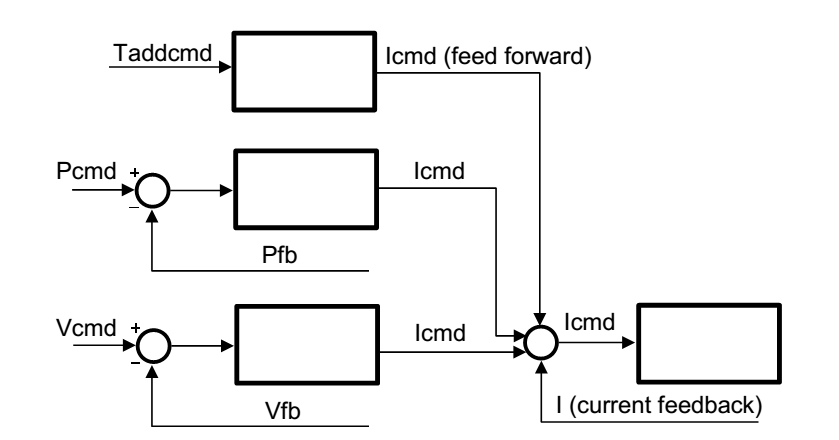
术语逆动力学模型(通常称为“转矩计算控制”)意味着softMC负责运动元素的笛卡尔运动,不仅计算下一个笛卡尔设定点的关节位置,还计算运动所需的关节力矩。 为了能够做到这一点,它需要一个动态模型–即运动元素的质量和惯性的模型。 关节速度和扭矩然后作为附加的扭矩命令数据发送到驱动器(见图1)。
在大多数情况下,用户没有动力学模型的参数。在这种情况下,可以使用softMC识别过程来估算这些参数。 softMC可以通过测量并估算一些常用机器人模型的动力学模型参数。 识别过程如下进行:当机器人被命令执行一定的运动时,记录运动参数和机器人内部马达扭矩。 然后,根据机器人模型和测量结果生成机器人的动力学模型的参数。
力矩单位
MKS单位制将力矩单位定义为[Nm](牛顿*米)。当涉及电机时,电机转矩通常建模为与电流成比例。因此,可以在每个系统中以不同的单位来定义力矩。本节介绍每个系统的力矩单位以及它们如何相互关联。
softMC通过驱动器读取电机的转矩,但不是[Nm]单位。 因此,softMC包含一个名为TorqueFactor(TFac)的轴属性,它将电机的转矩参数分开,以便将其转换为所需的单位。 该操作的结果存储在名为 TorqueFeedback的轴属性中。
CDHD驱动器设置
CDHD驱动器具有以下参数来定义电机的电流特性:
- MICONT – 以安培[A]为单位, 但是以毫安[mA]为单位读取,定义了电机的连续电流。这是长运行周期的最大允许值。
- MIPEAK – 以安培[A]为单位,但是以毫安[mA]为单位来读取,定义了电动机的峰值电流。 这是非常短的运行周期的最大允许值。
- MKT – 对旋转电机, 以[Nm/A]为单位读取, 定义了转矩常数,即电机每安培单位电机输出多少转矩。
- MKF – 对直线电机, 以[N/A]为单位读取, 定义了转矩常数,即电机每安培单位电机输出多少转矩。
- I – 以milli-MICONT [0.001 * MICONT]为单位读取。 它表示电流的实际值。它对应于电机中的电流。
TorqueFeedback属性计算如下:
因此,应该适当地设置TorqueFactor属性,以便将TorqueFeedback值转换为[Nm]:
100万是为了补偿MICONT单位是[mA],当前实际值是以[0.001 * MICONT]为单位。 通过这种方式定义TorqueFactor会将当前实际值转换为[Nm]的单位(并将该值分配给TorqueFeedback)。 在设置Tfac后,所有的扭矩值(Tfb,TCmd,Tmax,TorqueThreshold,Te)将始终以[Nm](线性轴为[N])为单位。 图2给出了在MC-Basic中这个计算的例子。
EtherCAT和CANopen标准(DS402)
EtherCAT标准定义了与上述参数等效的以下参数:
| CDHD 参数 | EtherCAT 参数 | EtherCat 索引 |
|---|---|---|
| MICONT | 电机额定电流 | 0x6075 |
| MIPEAK | 电机峰值电流 | 0x2036 |
| MKT | 力矩常数 | 0x2039 |
| MKF | 直线电机推力常数 | 0x2038 |
| I | 实际电流值 | 0x6078 |
softMC转矩相关属性
softMC具有以下转矩相关的属性:
- <axis>.TorqueThreshold - 轴转矩阈值,用于定义TADDCOMMAND值的限制。如果超过此值,softMC引发一个错误。可以将此值设置为用户所需的某个值,或设置为与驱动器MICONT或MIPEAK匹配的值。
例如,将TorqueThreshold设置为与MICONT匹配的值:
将TorqueThreshold设置为与MIPEAK匹配的值:
- <axis>.AdditiveTorqueDelay - 计算出的附加转矩指令基于pcmd 和vcmd。由于命令与轴的实际位置和速度之间存在延迟,所以相同的延迟应该被提供给附加转矩。AdditiveTorqueDelay用于此目的。该属性以循环时间为单位,它接受正整数值。AdditiveTorqueDelay工作如下:计算出的一定时间的附加转矩指令后只发送AdditiveTorqueDelay给驱动器。此属性的默认值是3。
如何包含传动比
通常,电机通过齿轮系统连接到关节。齿轮系统会影响电机所承受的扭矩负载,因此扭矩系数应该得到适当的补偿。经过补偿后,TorqueFactor参数将电流实际值参数从电机内部的电流([mMICONT]单位)转换为关节所承受的扭矩(单位[Nm])。
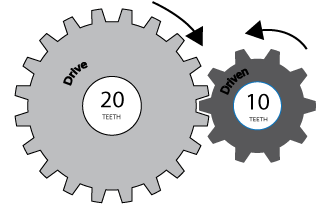
这里GR代表传动比。 图3显示了一个传动比的例子。
线性轴
以上所有都是指旋转轴。线性轴和旋转轴相比,是力而不是转矩。这些力以牛顿[N]为单位进行测量。因此,在处理线性轴时应进行一些修改。基本上有两种类型的直线轴 - 带有丝杠/滑轮/其他的旋转电机和直线电机。
带有丝杠/滑轮的旋转电机或用于将旋转运动转换为直线运动的不同类型的机构
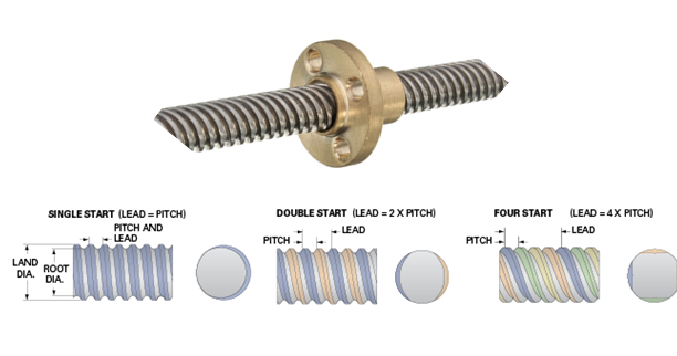
这种类型的处理与常规旋转轴一样进行单一修改。用于将旋转运动转换为线性运动的机制将由电机承载的扭矩负载转换为线性轴上的力负载。因此,TorqueFactor应该乘以另一个因子。此参数应包含旋转电机每转一圈(经过齿轮后)的直线运动量。对于丝杆,它将是丝杆导程[毫米/转]。对于一个滑轮,它将是滑轮的半径乘以2π[mm / rev]。TorqueFactor为:
SL代表丝杆导程或等效参数。 图4为一个丝杆导程的例子。
直线电机
这种类型与普通旋转轴的处理方式相同,但用 MKT 替换MKF属性,单位为[N/A],没有减速比, 因此TorqueFactor为:
操作模式和PDO
驱动器在使用动力学模型时的操作模式应该是周期同步位置模式。 动力学模型用于计算每台电机所需的转矩(或电流),但结果从来都不精确。 附加转矩指令仅用作第3节所述的前馈信号。
以下是使用动力学模型所必需的其他PDO(‘周期同步位置模式’PDO之外)的列表。:
| PDO 索引 | 描述 |
|---|---|
| RX: 0x60B2 | 转矩偏置 –附加转矩信号 |
| TX 0x6078 | 实际电流值 – 转矩反馈信号 |
如何进行动力学模型参数识别
数据采集
识别过程是通过移动机器人来记录运动参数和内部电机转矩。然后,根据机器人模型和测量结果,使用记录的数据来提取动力学模型参数。
高质量的数据对于获得良好的识别结果非常重要。高质量数据包含以不同速度和加速度分布在机器人运动空间的数据点。分散的数据为机器人的各种运动提供更好的参数拟合,从而可以高精度地预测附加转矩指令。
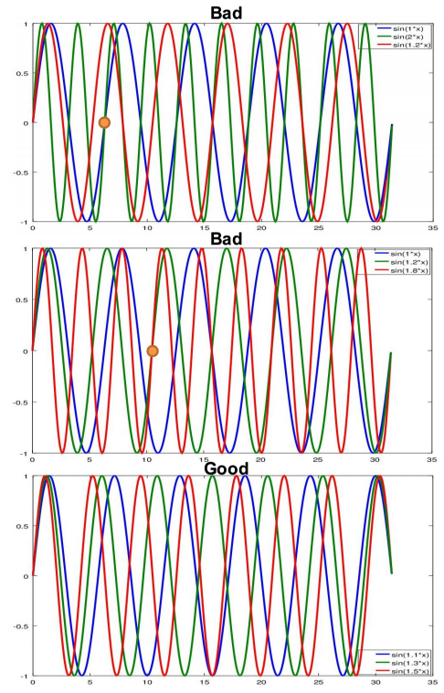
推荐的移动类型是使用正弦波命令。该命令以指定的幅度和频率移动机器人的每个关节。为了获得良好的离散数据,每个关节的振幅应接近其全部位置范围,每个关节的频率应与其他关节不同。每个关节的频率决定了关节之间运动的相关性。如果两个或多个关节具有相同的频率,则它们总是处于相同的相位,这将导致非离散的数据。此外,如果某个关节的频率是另一个关节的频率的倍数,那么在更快的关节的几个周期(更确切地说,乘法因子)之后将会重复相同的运动。实际上,对于任何合理的频率值,运动将在几个周期后重复。但是,为了获得良好的结果,建议每个关节至少获得三个周期的数据。因此,只要运动在这个记录时间内不重复,频率就选择好了。 以下是三种关节机器人的一些示例:
| J1 | J2 | J3 | 注释 | 质量 |
|---|---|---|---|---|
| 1 | 2 | 1.2 | j1和j2将在j1的1个周期和j2的2个周期之后重复 | Bad |
| 1 | 1.2 | 1.2 | j2和j3将在j2的3个周期和j3的2个周期之后重复 | Medium |
| 1.1 | 1.3 | 1.5 | j1,j2和j3 将在j1的11个周期,j2的13个周期和j3的15个周期之后重复 | Good |
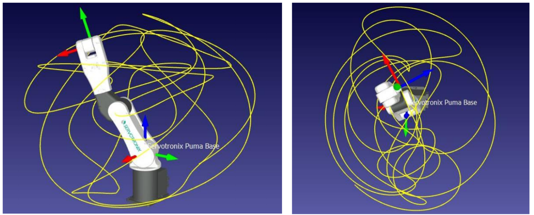
第一个例子不是一个好的频率选择,第二个例子是好的,最后一个例子是很好的参数选择。 显示这些正弦波组合的图表如图5所示。
最后,关节的速度也很重要。运动过程中的峰值速度应该接近每个关节的最大速度。在高速度下,动力学模型的加速度和速度对象是显着的,从而允许更准确的识别过程。关节的峰值速度可以通过运动的幅度和频率来调节。首先定义每个关节的振幅,然后设置一些任意的频率,例如{1.1,1.3,1.5},然后用一个标量因子乘以频率矢量:factor * {1.1,1.3,1.5}。通过改变因子,可以控制关节的速度。
识别任务的示例
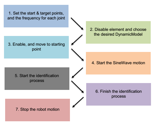
图6显示了识别过程的示意图。
执行识别过程的程序示例,该程序用于delta机器人:
1.  program
2.      dim startPoint as generic joint
3.      dim sineTarget as generic joint
4.      dim SWfreq as generic joint
5.
6.      startPoint = {-30,-30,-30,-200}
7.      sineTarget = {70,70,70,200}
8.      SWfreq = 0.3*{1,1.27,1.43,1.13}
9.
10.     with robot
11.         attach
11.	    En = 0
12.	    while En
13.	        sleep 100
14.	    end while
15.	    DynamicModel = 1
16.	    En = 1
17.	    while not En
18.	        sleep 100
19.	    end while
20.
21.	    Move startPoint Abs = 1
22.	    while IsMoving
23.	        sleep 100
24.	    end while
25.
26.	    SineWave sineTarget SineWaveFreq = SWfreq
27.	    sleep 2000
28.	' IdentFilterFreq is a Low pass filter.Frequency should be below 125 Hz
29.	    IdentificationStart IdentFilterFreq = 80
30.	' the time of the identification, you can change time.
31.	    sleep 20000
32.	    IdentificationFinish
33.
34.	    stop
35.	    while IsMoving
36.	        sleep 100
37.	    end while
38.	    proceed
39.	    En = 0
40.
41.	    detach
42.     end with
43. end program
这里是对示例程序的解释:
| 行号 | 描述 | ||||||||||
|---|---|---|---|---|---|---|---|---|---|---|---|
| 6 | 定义系统每个关节的起始位置 | ||||||||||
| 7 | 定义结束位置 | ||||||||||
| 8 | 定义每个关节的正弦波的频率(注意频率乘以因子0.3)。总的来说,这些是关节位置:
| ||||||||||
| 15 | 定义适合机器人的动力学模型,这将在稍后讨论。 请注意,只有在禁用机器人的情况下,才能修改此参数. | ||||||||||
| 21 | Moves the robot to the starting position | ||||||||||
| 26 | Starts the sinewave movement with the target – sineTarget and freque ncy – SWfreq | ||||||||||
| 29 | starts the recording of the data with the IdentificationStart command. At this line, one can also set a low pass filter over the collected data (over pfb and tfb) with a cutoff frequency set to IdentFilterFreq. The cutoff frequency must be larger than the largest sinewave frequency. One can try several cutoff frequencies and compare between the raw and filtered data, then choose the one that filters most of the noise without changing the real data. Please look for the identification wiki page for more information regarding the parameters that could be set for IdentificationStart command | ||||||||||
| 31 | sets a sleeping time – the recording time | ||||||||||
| 32 | stops the recording and apply the dynamic model parameters identification |
At the end of this task, a files named IDNT<group num>.PRG and IDNT<group num>.REC will be created in the MC folder.
The PRG file contains the identified parameters and the REC file contains the recorded data used for the identification.
The following subsections explain how to apply the identification for different robot models.
Identification process for different robot models
Single axis model
There are two types of single axis joints, linear and rotary. Each of these types has several different dynamic models as can be viewed in the Dynamic Models wiki page (and in section 5.4). Here are the different models in short:
Linear axis
The linear axis type has 2 dynamic model types:
- Horizontal axis
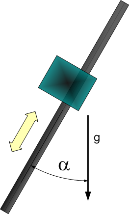
- Tilted axis – an axis with angle α relative to the vertical axis, ranging between 0 and 90 degrees (figure 7). When α = 0 the axis is vertical, and when α = 90 the axis is horizontal (the α parameter is found by the identification (i.e. it is not a user input).
Rotary axis
The rotary axis type has 3 dynamic model types:
- Simple rotary axis - which its center of mass is located on the rotation axis.
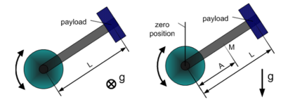
- Horizontal crank-arm axis (figure 8 left).
- Vertical crank-arm axis (figure 8 right).
Example for an identification task that will work for all types mentioned above:
1.  program
2.      dim startPoint as generic joint
3.      dim sineTarget as generic joint
4.      dim SWfreq as generic joint
5.
6.      startPoint = -350
7.      sineTarget = 350
8.      SWfreq = 1.5
9.
10.     with axis
11.         attach
11.	    En = 0
12.	    while En
13.	        sleep 100
14.	    end while
15.	    DynamicModel = 2
16.	    En = 1
17.	    while not En
18.	        sleep 100
19.	    end while
20.
21.	    Move startPoint Abs = 1
22.	    while IsMoving
23.	        sleep 100
24.	    end while
25.
26.	    SineWave sineTarget SineWaveFreq = SWfreq Abs = 1
27.	    sleep 2000
28.	' IdentFilterFreq is a Low pass filter.Frequency should be below 125 Hz
29.	    IdentificationStart IdentFilterFreq = 80
30.	' the time of the identification, you can change time.
31.	    sleep 20000
32.	    IdentificationFinish
33.
34.	    stop
35.	    while IsMoving
36.	        sleep 100
37.	    end while
38.	    proceed
39.	    En = 0
40.
41.	    detach
42.     end with
43. end program
To reuse this code, remember to use frequency and amplitude values that are suited for the application, and also use the suitable dynamic model type.
SCARA robot
The SARA robot has two kinematic models, one with 3 axes (XYZ) and the other with four axes (XYZR).
However, there is only one type of dynamic model which fits both of these kinematics models.
Example for an identification task that will work for 3 axes SCARA:
1.  program
2.      dim startPoint as generic joint
3.      dim sineTarget as generic joint
4.      dim SWfreq as generic joint
5.
6.      startPoint = {-160,-160,0}
7.      sineTarget = {160,160,150}
8.      SWfreq = 0.3*{1,1.27,1.43}
9.
10.     with SCARA
11.         attach
11.	    En = 0
12.	    while En
13.	        sleep 100
14.	    end while
15.	    DynamicModel = 1
16.	    En = 1
17.	    while not En
18.	        sleep 100
19.	    end while
20.
21.	    Move startPoint Abs = 1
22.	    while IsMoving
23.	        sleep 100
24.	    end while
25.
26.	    SineWave sineTarget SineWaveFreq = SWfreq
27.	    sleep 2000
28.	' IdentFilterFreq is a Low pass filter.Frequency should be below 125 Hz
29.	    IdentificationStart IdentFilterFreq = 80
30.	' the time of the identification, you can change time.
31.	    sleep 20000
32.	    IdentificationFinish
33.
34.	    stop
35.	    while IsMoving
36.	        sleep 100
37.	    end while
38.	    proceed
39.	    En = 0
40.
41.	    detach
42.     end with
43. end program
Example for an identification task that will work for 4 axes SCARA:
1.  program
2.      dim startPoint as generic joint
3.      dim sineTarget as generic joint
4.      dim SWfreq as generic joint
5.
6.      startPoint = {-160,-160,0,-350}
7.      sineTarget = {160,160,150,350}
8.      SWfreq = 0.3*{1,1.27,1.43,1.13}
9.
10.     with SCARA
11.         attach
11.	    En = 0
12.	    while En
13.	        sleep 100
14.	    end while
15.	    DynamicModel = 1
16.	    En = 1
17.	    while not En
18.	        sleep 100
19.	    end while
20.
21.	    Move startPoint Abs = 1
22.	    while IsMoving
23.	        sleep 100
24.	    end while
25.
26.	    SineWave sineTarget SineWaveFreq = SWfreq
27.	    sleep 2000
28.	' IdentFilterFreq is a Low pass filter.Frequency should be below 125 Hz
29.	    IdentificationStart IdentFilterFreq = 80
30.	' the time of the identification, you can change time.
31.	    sleep 20000
32.	    IdentificationFinish
33.
34.	    stop
35.	    while IsMoving
36.	        sleep 100
37.	    end while
38.	    proceed
39.	    En = 0
40.
41.	    detach
42.     end with
43. end program
To reuse this code, remember to use frequency and amplitude values that are suited for the application.
Some SCARA robots have coupled joints, usually the 3rd and 4th joints. Currently, the dynamic model of the SCARA robot does not take the coupling into account. Therefore, there may be large errors for coupled joints
DELTA robot
The Delta robot has two kinematic models, one with 3 axes (XYZ) and the other with four axes (XYZR).
However, there is only one type of dynamic model which fits both of these kinematics models.
Example for an identification task that will work for 3 axes Delta:
1.  program
2.      dim startPoint as generic joint
3.      dim sineTarget as generic joint
4.      dim SWfreq as generic joint
5.
6.      startPoint = {-30,-30,-30}
7.      sineTarget = {70,70,70}
8.      SWfreq = 0.3*{1,1.27,1.43}
9.
10.     with DELTA
11.         attach
11.	    En = 0
12.	    while En
13.	        sleep 100
14.	    end while
15.	    DynamicModel = 1
16.	    En = 1
17.	    while not En
18.	        sleep 100
19.	    end while
20.
21.	    Move startPoint Abs = 1
22.	    while IsMoving
23.	        sleep 100
24.	    end while
25.
26.	    SineWave sineTarget SineWaveFreq = SWfreq
27.	    sleep 2000
28.	' IdentFilterFreq is a Low pass filter.Frequency should be below 125 Hz
29.	    IdentificationStart IdentFilterFreq = 80
30.	' the time of the identification, you can change time.
31.	    sleep 20000
32.	    IdentificationFinish
33.
34.	    stop
35.	    while IsMoving
36.	        sleep 100
37.	    end while
38.	    proceed
39.	    En = 0
40.
41.	    detach
42.     end with
43. end program
Example for an identification task that will work for 4 axes Delta:
1.  program
2.      dim startPoint as generic joint
3.      dim sineTarget as generic joint
4.      dim SWfreq as generic joint
5.
6.      startPoint = {-30,-30,-30,-350}
7.      sineTarget = {70,70,70,350}
8.      SWfreq = 0.3*{1,1.27,1.43,1.13}
9.
10.     with DELTA
11.         attach
11.	    En = 0
12.	    while En
13.	        sleep 100
14.	    end while
15.	    DynamicModel = 1
16.	    En = 1
17.	    while not En
18.	        sleep 100
19.	    end while
20.
21.	    Move startPoint Abs = 1
22.	    while IsMoving
23.	        sleep 100
24.	    end while
25.
26.	    SineWave sineTarget SineWaveFreq = SWfreq
27.	    sleep 2000
28.	' IdentFilterFreq is a Low pass filter.Frequency should be below 125 Hz
29.	    IdentificationStart IdentFilterFreq = 80
30.	' the time of the identification, you can change time.
31.	    sleep 20000
32.	    IdentificationFinish
33.
34.	    stop
35.	    while IsMoving
36.	        sleep 100
37.	    end while
38.	    proceed
39.	    En = 0
40.
41.	    detach
42.     end with
43. end program
To reuse this code, remember to use frequency and amplitude values that are suited for the application.
PUMA robot
The PUMA robot has only one kinematic model but it has two different dynamic models.
The first dynamic model is a regular model like the other robots.
The second model is a semi-static model, meaning it will work only for slow movements and static positions. This model takes into account only the gravity and friction forces / torques.
Full regular model
This model identification rules are just like the previous models.
Example for an identification task that will work for PUMA:
1.  program
2.      dim startPoint as generic joint
3.      dim sineTarget as generic joint
4.      dim SWfreq as generic joint
5.
6.      startPoint = {-100,-170,100,-60,-60,-100}
7.      sineTarget = {100,-40,235,60,60,100}
8.      SWfreq = 0.15*{1.56,1,1.31,1.47,1.21,1.17}
9.
10.     with PUMA
11.         attach
11.	    En = 0
12.	    while En
13.	        sleep 100
14.	    end while
15.	    DynamicModel = 1
16.	    En = 1
17.	    while not En
18.	        sleep 100
19.	    end while
20.
21.	    Move startPoint Abs = 1
22.	    while IsMoving
23.	        sleep 100
24.	    end while
25.
26.	    SineWave sineTarget SineWaveFreq = SWfreq
27.	    sleep 2000
28.	' IdentFilterFreq is a Low pass filter.Frequency should be below 125 Hz
29.	    IdentificationStart IdentFilterFreq = 80
30.	' the time of the identification, you can change time.
31.	    sleep 20000
32.	    IdentificationFinish
33.
34.	    stop
35.	    while IsMoving
36.	        sleep 100
37.	    end while
38.	    proceed
39.	    En = 0
40.
41.	    detach
42.     end with
43. end program
To reuse this code, remember to use frequency and amplitude values that are suited for the application.
Semi-static model
The semi-static model identification is a little bit different from all of the examples so far. This model takes into account only gravity and friction forces, in other words it neglects dynamic forces. Therefore, the measurement should include negligible dynamic forces, and this is possible by moving slow.
This identification process is longer than the usual identification progress, it takes approximately 2-3 minutes. In addition, it is advised to perform less than 3 cycles, 1 cycle should be enough.
Also, similar to the previous examples, the semi-static model threshold the velocity of the data points. But unlike the previous examples, here there are two thresholds, one for avoiding very low velocities avoiding numeric errors) and the other for avoiding high velocities (avoiding significant dynamic forces).
Example for such an identification process:
1.  program
2.      dim startPoint as generic joint
3.      dim sineTarget as generic joint
4.      dim SWfreq as generic joint
5.
6.      startPoint = {-100,-170,100,-60,-60,-100}
7.      sineTarget = {100,-40,235,60,60,100}
8.      SWfreq = 0.02*{1.56,1,1.31,1.47,1.21,1.17}
9.
10.     with PUMA
11.         attach
11.	    En = 0
12.	    while En
13.	        sleep 100
14.	    end while
15.	    DynamicModel = 1
16.	    En = 1
17.	    while not En
18.	        sleep 100
19.	    end while
20.
21.	    Move startPoint Abs = 1
22.	    while IsMoving
23.	        sleep 100
24.	    end while
25.
26.	    SineWave sineTarget SineWaveFreq = SWfreq
27.	    sleep 2000
28.	' IdentFilterFreq is a Low pass filter.Frequency should be below 125 Hz
29.	    IdentificationStart IdentFilterFreq = 80
30.	' the time of the identification, you can change time.
31.	    sleep 20000
32.	    IdentificationFinish
33.
34.	    stop
35.	    while IsMoving
36.	        sleep 100
37.	    end while
38.	    proceed
39.	    En = 0
40.
41.	    detach
42.     end with
43. end program
Note the significant low frequencies which cause slow movement.
The Dynamic Models Parameters
This section lists the dynamic parameters for each type of dynamic model.
Rotary Axis
Dynamic Model 1 – simple rotary axis
| Number | Parameter | Comments |
|---|---|---|
| 1 | Total moment of inertia around the rotation axis of the moved part |
- Model equation
Dynamic Model 2 - horizontal crank-arm axis
| Number | Parameter | Comments |
|---|---|---|
| 1 | Total moment of inertia around the rotation axis of the moved part | |
| 2 | Square of length of crank arm (axis to payload) |
- Model equation
Dynamic Model 3 - vertical crank-arm axis
| Number | Parameter | Comments |
|---|---|---|
| 1 | Total moment of inertia around the rotation axis of the moved part | |
| 2 | Square of length of crank arm (axis to payload) | |
| 3 | Mass (without payload) * Gravity * Distance to center of mass | |
| 4 | Gravity * Distance to Payload |
- Model equation
Linear Axis
Dynamic Model 1 - horizontal axis
| Number | Parameter | Comments |
|---|---|---|
| 1 | Total mass of the moved part. |
- Model equation
Dynamic Model 2 - vertical or tilted axis
| Number | Parameter | Comments |
|---|---|---|
| 1 | Total mass of the moved part. | |
| 2 | Constant force due to gravity. | |
| 3 | Gravity coefficient used to consider payload mass. (g = 9.80665) |
- Model equation
SCARA robot
Dynamic Model 1
| Number | Parameter | Comments |
|---|---|---|
| 1 | ||
| 2 | ||
| 3 | ||
| 4 | ||
| 5 | ||
| 6 | ||
| 7 | ||
| 8 |
DELTA robot
Dynamic Model 1
| Number | Parameter | Comments |
|---|---|---|
| 1 | kg*m2 | |
| 2 | kg*m2/sec2 | |
| 3 | kg | |
| 4 | kg*m2 | |
| 5 | kg | |
| 6 | kg | |
| 7 | kg*m2 | |
| 8 | kg*m2 | |
| 9 | m | |
| 10 | m | |
| 11 | ||
| 12 | ||
| 13 | ||
| 14 |
PUMA robot
Dynamic Model 1
Description:
- - Gravity constant
- - Mass of the ith link
- - length of the common normal between the ith and ith+1 joints
- - offset along z axis between the ith and ith+1 joints
- - The distance from the ith joint to the center of mass of the ith link
| Number | Parameter | Comments |
|---|---|---|
| 1 | |
kg/m^2 |
| 2 | kg/m^2 | |
| 3 | kg/m^2 | |
| 4 | kg/m^2 | |
| 5 | kg/m^2 | |
| 6 | kg/m^2 | |
| 7 | kg/m^2 | |
| 8 | kg/m^2 | |
| 9 | kg/m^2 | |
| 10 | kg/m^2 | |
| 11 | kg/m^2 | |
| 12 | kg/m^2 | |
| 13 | kg/m^2 | |
| 14 | kg/m^2 | |
| 15 | kg/m^2 | |
| 16 | kg/m^2 | |
| 17 | kg/m^2 | |
| 18 | kg/m^2 | |
| 19 | kg/m^2 | |
| 20 | kg/m^2 | |
| 21 | kg/m^2 | |
| 22 | kg/m^2 | |
| 23 | kg/m^2 |
Dynamic Model 2 - Gravity
| Number | Parameter | Comments |
|---|---|---|
| 1 | kg*m^2/s^2 | |
| 2 | kg*m^2/s^2 | |
| 3 | kg*m^2/s^2 | |
| 4 | kg*m^2/s^2 |
Identification with a Payload
The IdentificationStart command has a boolean parameter called ‘IdentPayload’. If this parameter is set to false, the identification process is performed regularly. If this parameter is set to true, the identification process identifies only the payload mass or inertia.
In order to identify the payload, one must follow these steps:
- Perform an identification process without the payload.
- Set the dynamic model parameters (by running the identification PRG file).
- Set ‘IdentPayload’ to true and perform an identification process with the payload.
| NOTE | |
| After performing an identification process with the payload and setting ‘IdentPayload’ to true, the identification PRG file will contain the dynamic model parameters form step 1, and the payload parameters from step 3 |
| NOTE | |
| This procedure is valid to all dynamic models except dynamic model 1 of the PUMA robot. |
Explanation of the identification output file
Example of an identification output PRG file. The file is generated at the end of the identification process, and is named: IDNT<group num>.PRG:
1. 'Dynamic parameter identification for PUMA succeeded!
2. 'Identification date and time: 29/03/17 08:17:08
3. 'Max relative torque error: axis 1 = 13.86 %; axis 2 = 8.70 %; axis 3 = 7.79 %; axis 4 = 17.87 %; axis 5 = 23.87 %; axis 6 = 43.85 %; (maximal allowed = 50.00 %)
4. 'Mean relative torque error: axis 1 = 3.18 %; axis 2 = 1.71 %; axis 3 = 1.88 %; axis 4 = 3.59 %; axis 5 = 5.88 %; axis 6 = 12.41 %;
5. 'Signal filter cutoff frequency = 20.000 Hz
6. 'Signal data length = 49876 samples (raw record length = 50000 samples)
7. 'Moving data length: axis 1 = 35998 samples (threshold = 0.038770 rad/s); axis 2 = 35405 samples (threshold = 0.031481 rad/s); axis 3 = 36032 samples (threshold = 0.039294 rad/s); axis 4 = 36785 samples (threshold = 0.041069 rad/s); axis 5 = 34931 samples (threshold = 0.038757 rad/s); axis 6 = 29759 samples (threshold = 0.062830 rad/s);

8.  PROGRAM CONTINUE
9.  ATTACH PUMA

10. PUMA.DynamicParameter[1] = 8.759309007e+01
11. PUMA.DynamicParameter[2] = 1.021832253e+01
12. PUMA.DynamicParameter[3] = 3.042091725e+01
13. PUMA.DynamicParameter[4] = 1.560383089e+00
14. PUMA.DynamicParameter[5] = 0.000000000e+00
15. PUMA.DynamicParameter[6] = 0.000000000e+00

16. A1.ViscousFriction = -1.547427791e+02
17. A1.CoulombFriction = -2.018153298e+01

18. A2.ViscousFriction = -1.603287029e+02
19. A2.CoulombFriction = -4.658045702e+01

20. A3.ViscousFriction = -1.085257604e+02
21. A3.CoulombFriction = -1.961987594e+01

22. A4.ViscousFriction = -1.142833743e+01
23. A4.CoulombFriction = -9.124446870e+00

24. A5.ViscousFriction = -2.468491129e+01
25. A5.CoulombFriction = -3.713111266e+00

26. A6.ViscousFriction = -2.173025205e+00
27. A6.CoulombFriction = -9.724658207e-01

29. PUMA.DynamicModel = 2

30. DETACH PUMA
31. TERMINATE PROGRAM
Line 1-7 give information about the identification process. Line 1 reports if the identification was successful or not.
2. 'Identification date and time: 29/03/17 08:17:08
3. 'Max relative torque error: axis 1 = 13.86 %; axis 2 = 8.70 %; axis 3 = 7.79 %; axis 4 = 17.87 %; axis 5 = 23.87 %; axis 6 = 43.85 %; (maximal allowed = 50.00 %)
Line 2 reports the date and time the identification was made.
Line 3 reports the recorded max relative torque error. The torque error is taken as the TorqueAdditiveCommand (Taddcmd) minus the measured TorqueFeedback. The Taddcmd for this calculation is taken as the Taddcmd that would have been calculated with the identified dynamic parameters as if this movement was performed. In other words, the error is the difference between the real data and the fitted model. The relative torque error is calculated as the torque error divided by the max measured TorqueFeedback (each joint and its max TorqueFeedback value). The max relative torque error, is the maximum value of the relative value for each joint. The formula for the max relative torque error is:
If this value is larger than 50% for one of the joints than the identification is regarded as failed.
4. 'Mean relative torque error: axis 1 = 3.18 %; axis 2 = 1.71 %; axis 3 = 1.88 %; axis 4 = 3.59 %; axis 5 = 5.88 %; axis 6 = 12.41 %;
5. 'Signal filter cutoff frequency = 20.000 Hz
6. 'Signal data length = 49876 samples (raw record length = 50000 samples)
Line 4 reports the mean relative torque error, the mean of the relative torque error over all of the recorded time is taken and displayed for each joint.
Line 5 reports the cutoff frequency that was used for the low pass filter.
Line 6 reports how many data points were recorded.
7. 'Moving data length: axis 1 = 35998 samples (threshold = 0.038770 rad/s); axis 2 = 35405 samples (threshold = 0.031481 rad/s); axis 3 = 36032 samples (threshold = 0.039294 rad/s);
'axis 4 = 36785 samples (threshold = 0.041069 rad/s); axis 5 = 34931 samples (threshold = 0.038757 rad/s); axis 6 = 29759 samples (threshold = 0.062830 rad/s);
Line 7 reports how many data points from each joint were taken for the model fitting. Some data points are discarded if the velocity of the joint in these point is below some threshold (the threshold for each joint is also reported in this line). This is done because the data points with low velocities are causing numerical errors to the model fitting. Therefore, all of the relative errors explained above are calculated only for those points which are taken into account for the model fitting.
10. PUMA.DynamicParameter[1] = 8.759309007e+01
11. PUMA.DynamicParameter[2] = 1.021832253e+01
12. PUMA.DynamicParameter[3] = 3.042091725e+01
13. PUMA.DynamicParameter[4] = 1.560383089e+00
14. PUMA.DynamicParameter[5] = 0.000000000e+00
15. PUMA.DynamicParameter[6] = 0.000000000e+00
Lines 10-15 (for this file) sets the fitted dynamic model parameters.
16. A1.ViscousFriction = -1.547427791e+02
17. A1.CoulombFriction = -2.018153298e+01
18. A2.ViscousFriction = -1.603287029e+02
19. A2.CoulombFriction = -4.658045702e+01
20. A3.ViscousFriction = -1.085257604e+02
21. A3.CoulombFriction = -1.961987594e+01
22. A4.ViscousFriction = -1.142833743e+01
23. A4.CoulombFriction = -9.124446870e+00
24. A5.ViscousFriction = -2.468491129e+01
25. A5.CoulombFriction = -3.713111266e+00
26. A6.ViscousFriction = -2.173025205e+00
27. A6.CoulombFriction = -9.724658207e-01
Lines 16-27 (for this file) sets the fitted friction parameters.
29. PUMA.DynamicModel = 2
Line 29 (for this file) sets the dynamic model that was used for this identification process.
Success condition
The success condition is based on the relative torque error. Each axis should have a max relative torque error value below 50% in order for the identification to be considered as successful.
The torque error is taken as the TorqueAdditiveCommand (Taddcmd) minus the measured TorqueFeedback. The Taddcmd for this calculation is taken as the Taddcmd that would have been calculated with the identified dynamic parameters as if this movement was performed. In other words, the error is the difference between the real data and the fitted model.
The relative torque error is calculated as the torque error divided by the max measured TorqueFeedback (each joint and its max TorqueFeedback value). The max relative torque error, is the maximum value of the relative value for each joint. If this value is larger than 50% for one of the joints than the identification is regarded as failed. Line 4 reports the mean relative torque error, the mean of the relative torque error over all of the recorded time is taken and displayed for each joint. Please note that the relative torque error is evaluated only for the points that stand in a minimum velocity limitation.
The max relative torque error may vary between the different joint. Typically, small joints (with small motors) have larger relative error. This is because the applied torque for these motors is small and the noise in measurement is in the same order of magnitude of the applied torque.
For example: Let’s assume that for a certain point j1.TorqueFeedback = 80 and the j1.TorqueAdditiveCommand = 100. For this point, the j1.TorqueError = 20. Let’s assume that the maximum j1.TorqueFeedback during the recording was 160, then the relative torque error for this point would be: j1.TorqueError/max(j1.TorqueFeedback) = 20/160 = 0.125 = 12.5%
Parameters
Robot models which are supported for dynamic model, have at least one type of dynamic model. These models can be found in the wiki page Dynamic Models. Each model is based on some parameters which are composed of the mass, length and inertia of the different parts of the robot. These are the parameters that are being evaluated with the help of the identification process. The parameters are saved as robot.DynamicParameter[i], where robot is the robot name and i is the number of the parameter as stated in the Dynamic Models page. Each model may have different number of parameters.
After the dynamic parameter, appear the viscous friction and coulomb friction parameters: axis.ViscousFriction, axis.CoulombFriction . Each joint of the robot has these two parameters which define its friction coefficients.
In addition to these parameters, the user should consider to set the maximum allowed value for the additive torque command. This could be set with the property TorqueThreshold, e.g. a1.TorqueThreshold = 200. If the Taddcmd exceeds this value, than the softMC reports an error.
Including the identification output file in setup
In order for the dynamic model to take effect you should simply run the IDNT<group num>.PRG file while the robot is disabled (en = 0). Note that this should come after the robot setup. In order to automatically load the dynamic model configuration during the system initialization and robot setup, simply add the line:
Load IDNT<group num>.PRG To the end of your AUTOEXEC.PRG or STARTPRG.PRG file, after the robot setup.
Explanation of the identification process recording file
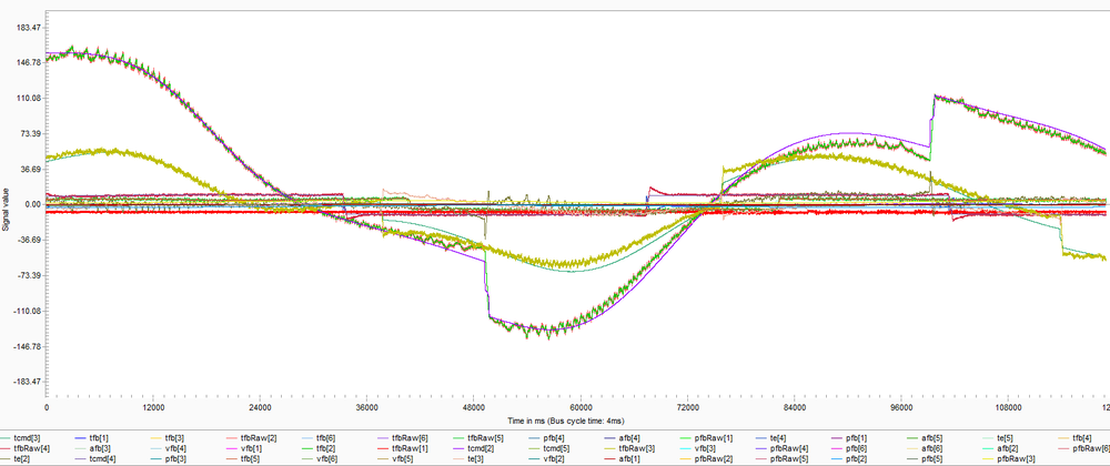
Another file that is generated at the end of the identification process is the data recording file. This file is named: IDNT<group num>.REC. This file contains all of the relevant data that was used by the identification process. Here are the parameters which are displayed for each joint:
- tfbRaw – The raw recorded data of the TorqueFeedback (tfb) property.
- pfbRaw – The raw recorded data of the PositionFeedback (pfb) property.
- tfb – The filtered recorded data of the TorqueFeedback (tfb) property.
- pfb – The filtered recorded data of the PositionFeedback (pfb) property.
- vfb – The filtered recorded data of the VelocityFeedback (vfb) property.
- afb – The filtered recorded data of the AccelerationFeedback (afb) property.
- tcmd – The torque command generated by the fitted model. The found dynamic parameters and the collected data are used to calculate this property. In regular mode, this property will actually be TorqueAdditiveCommand (Taddcmd).
- te – The TorqueError (te) calculated by the difference of the tcmd and tfb data.
This file can be used for better debugging and troubleshooting, as well as for better understanding the identification process. At figure 15 you can find example of an identification output REC file:
Demonstration of tracking improvements (settling, position error)
SCARA Robot
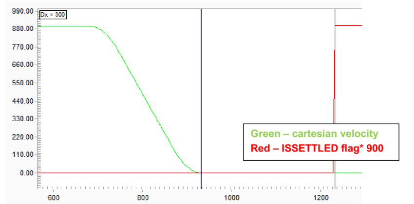
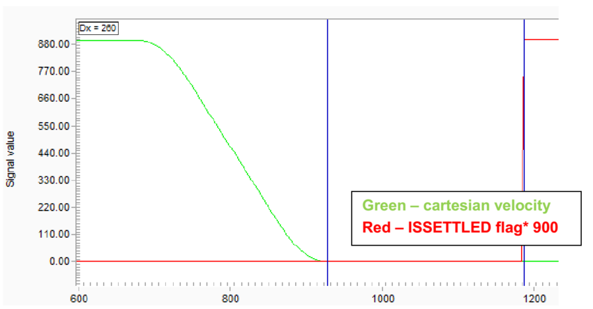
An experiment was made for a 4 axes scara robot with and without dynamic model. The robot was commanded to move 600[mm] in a straight line with linear velocity of 900[mm/s]. The cartesian velocity of the robot and the ISSETTLED property were recorded during this motion (figure 16 and 17, the ISSETTLED property is scaled by 3000).
The ISSETTLED property indicates whether the actual element position is within the specified settling range. The settling range is defined by the PESETTLE property and is further qualified by the TIMESETTLE property. When the motion profiler has completed, the absolute value of the position error (Target Position – Actual Position) is compared to the PESETTLE property. When the result is less than or equal to this property for the time given by TIMESETTLE, the ISSETTLED flag is set. For this example, the PESETTLE was taken as 0.001.
Therefore, one could expect that a shorter settling time indicates on better performance.
Figures 16 and 17 display the recorded data from the experiment. The results are that the settling time for this motion without dynamic model is 300 ms, and the settling time with dynamic model is 260 ms – ~86.7% of the original settling time.
DELTA Robot
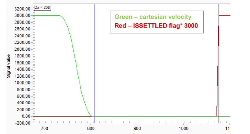
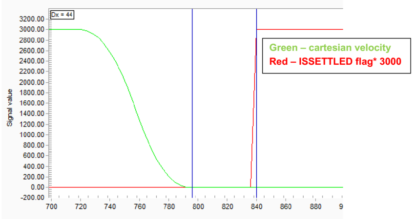
An experiment was made for a 3 axes delta robot with and without dynamic model. The robot was commanded to move 550[mm] in a straight line with linear velocity of 3000[mm/s]. The cartesian velocity of the robot and the ISSETTLED property were recorded during this motion (figure 17 and 18, the ISSETTLED property is scaled by 3000).
The ISSETTLED property indicates whether the actual element position is within the specified settling range. The settling range is defined by the PESETTLE property and is further qualified by the TIMESETTLE property. When the motion profiler has completed, the absolute value of the position error (Target Position – Actual Position) is compared to the PESETTLE property. When the result is less than or equal to this property for the time given by TIMESETTLE, the ISSETTLED flag is set. For this example, the PESETTLE was taken as 0.05.
Therefore, one could expect that a shorter settling time indicates on better performance.
Figures 17 and 18 display the recorded data from the experiment. The results are that the settling time for this motion without dynamic model is 268 ms, and the settling time with dynamic model is 44 ms – ~16.5% of the original settling time.
PUMA Robot
An experiment was made with and without dynamic model. Axis 3 was commanded to oscillate with the SineWave command while axis 2 was commanded to stay at 0.
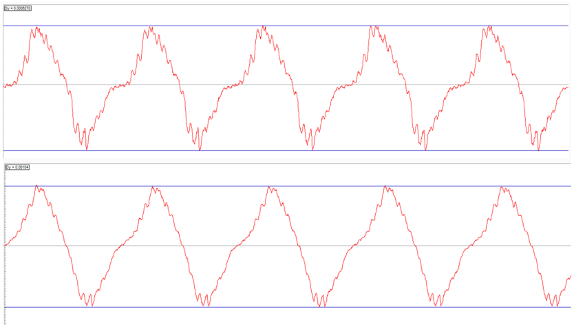
Figure 19 shows axis 2 position error for the cases with (top) and without (bottom) dynamic model. The peak to peak amplitude for the cases with and without dynamic model are ~0.6e-3 and ~1e-3 correspondingly. It means that using the dynamic model reduced ~40% of the error for this example.
Collision detection
The dynamic model allows to enable a more delicate collision detection feature. Without the dynamic model, the softMC can detect a collision by thresholding the position error of the robot or joints. However, when using the dynamic model of the robot, a collision can be detected by thresholding the torque error. The torque error reacts quicker than the position error, hence enabling a more delicate collision detection.
In order to activate the thresholding over the torque error for a certain joint, set the property TorqueErrorEnable (Teen) to 1, e.g. a1.Teen = 1. One more property to set is the TorqueErrorMax (Temax), e.g. a1.Temax = 10. This property set the maximum allowed torque error which above it softMC reports an error. Note that the Temax property may vary between joints, usually the bigger the joint’s motor the bigger Temax that the user should allow. Also note that as the dynamic model identification results get more accurate, the Temax can be decreased as the torque error gets smaller.
One last property to consider is the TorqueErrorFilter property. If the torque feedback is noisy, the Temax value can be exceed due to noise which causes false collision triggering. Filtering this noise helps to achieve better collision detection procedure. This property gets values in the range of 0.0 to 1.0. The filter is a very simple averaging filter, it performs as follows:
when TE is the TorqueError property, and TEF is the TorqueErrorFilter property.
Note that usually the largest error occurs in the beginning, ending or direction changing of the movement. Therefore, the magnitude of the errors in these cases determine what the Temax value will be. Nevertheless, these cases are also characterized with very low velocities. Hence, it is possible to write an application that monitors the torque error and joint velocities, and ignore the cases when the velocity is small, or perhaps increase the Temax just for these cases. As a result, the collision detection feature can become very sensitive
Review of the possible reasons for an identification failure
This section reviews some possible reasons that may cause poor results or a failure of the identification process. The next section reviews how to identify these reasons.
Movement is too slow
The dynamic identification model requires that the robot joints will move in a high velocity, as mentioned in section 3. When the joints move at a low velocity, the developed torque in the joints opposes mainly the joints friction and gravity torques, and the acceleration and inertia terms are relatively small. Therefore, the dynamic model parameters identification will perform poorly. Furthermore, the identification process ignores data that is under certain minimal velocity, so moving slowly can also cause for lack of data.
That being said, in such a case, the output PRG identification file may report that the identification process was successful and the resulting max relative errors can be small. However, later, when attempting to move at higher velocities than the velocities used during the identification process, the additive torque command predictions will most likely perform poorly.
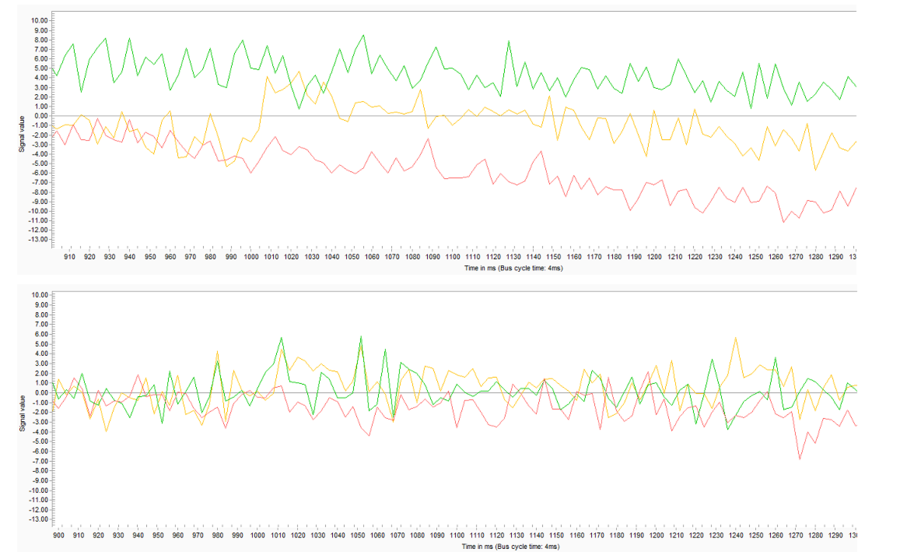
Figure 20 shows an example for an identification output REC file for a 3 axes delta robot where the motion was slow during the identification. It is noticeable that the data is very noisy. The reason for that is that the movement is slow, hence the developed torques are small and the relative noise is large
Figure 21 shows the torque error for the same delta robot and the same motion. The top figure is the result of the motion using the retrieved parameters from a slow identification process and the bottom figure is the result of the motion using the retrieved parameters from a good identification process. One can see that the torque errors increase dramatically for the case with slow identification process
Movement is too fast
This problem is less likely to happen, but still, it can cause poor results or a failure of the identification process.
If the robot joints are brought to their limits, the motor torque can reach to a saturation value. The current dynamic model does not take saturation into account, therefore, if saturation occurred, it will cause poor identification results
Movement duration is too short
The identification is based on the collected data that is recorded during the robot movement. If there is not enough data, the identification may overfit the data and will predict accurately just for the region of the collected data. In such case the identification may be reported as successful, hence the user has to judge if the collected data is sufficient. A rule of thumb is that each joint should complete at least 3 cycles.
Movement region is too small
The identification is based on the collected data that is recorded during the robot movement. If the data is not scattered over the entire work area of the robot, the identification may overfit the data and will predict accurately just for the region of the collected data.
In such case the identification may be reported as successful, hence the user has to judge if the collected data is sufficient. A rule of thumb is that each joint should reach position values closely to its negative and positive position limits.
TorqueFactor properties are not configured well
The dynamic model of each robot is based on the MKS system of units defines, hence the torque feedback values should be in units of [Nm]. If the TorqueFactor properties are not configured well than the torque feedback will not have suitable values and the model equations will be wrong.
In such a case, the identification process will perform poorly and the identified model parameters will not be correct.
Wrong type of DynamicModel property
Some kinematic models are assigned with more than one type of dynamic model. These different models are in order to deal with different configurations. For example, a linear axis may be horizontal, vertical, or tilted in a certain angle, each of those configurations has a different dynamic model and different DynamicModel property value.
If a wrong DynamicModel value is set, the identification process will perform poorly.
How to assess what is the failure reason based on the output files
This section reviews some possible failure results of the generated identification files and the identification process. The failures may be the failure of the identification process, or successful identification process with poor performance results.
Identification process failure
An identification failure is the case where one of the joints results with a max relative error larger than 50%. Here are some reasons that may cause this result:
- One or more of the joints moved too slow. This can be identified in the output PRG file in lines 6 and 7. Line 6 reports how many data points were collected for each joint. Line 7 reports how many points are with a velocity larger than the velocity threshold. If the data points number after thresholding for one or more of the joints is significantly smaller than the total number of collected points, then it means that this joint moved too slow.
- One or more of the joints reached saturation. This can be identified in the output REC file. Open the output REC file and observe only the following properties of the joint in subject: tfb, tcmd and te. Saturation can be identified by seeing that the tfb reaches a sudden plateau while the tdcmd continues regularly.
- Large noise for small joints. For some systems, the noise can be in the same order of magnitude of the mean operation currents. In such cases, the

