Difference between revisions of "AXY:MC Operational Modes"
| Line 44: | Line 44: | ||
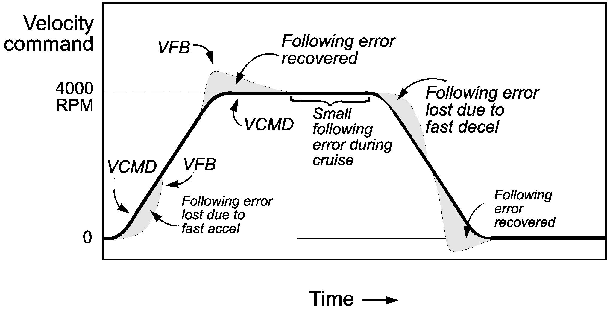
When GVFR is at full scale (GVFR =1), the following error at steady-state is reduced to zero. The only following error is generated during transients. The effect of full feed-forward on following error is shown in the following figure. | When GVFR is at full scale (GVFR =1), the following error at steady-state is reduced to zero. The only following error is generated during transients. The effect of full feed-forward on following error is shown in the following figure. | ||
| − | <center>[[Image | + | <center>[[Image:Axystems;MC_Operational_Modes_Velocity_Command.jpg]]</center> |
<center>''Following Error with Proportional Loop and Feed-Forward''</center> | <center>''Following Error with Proportional Loop and Feed-Forward''</center> | ||
Revision as of 09:23, 1 February 2011
Loop Types
The AMCS system supports the next main control loop types:
- Position Control with standard feedback. This is OPMODE 5.
- Position Control with Dual-feedback (OPMODE 5)
- Position Loop Feedback from external feedback (load sensor) . (OPMODE 5)
- Digital Velocity Control with standard feedback (motor sensor). This is OPMODE 0.
- Analog Velocity Control. This is OPMODE 1.
- Digital Torque. This is OPMODE 2.
- Analog Torque. This is OPMODE 3.
The AMCS sends position and velocity commands each update cycle. The operation of the
AMCS is hardly affected by the loop selection. The loop selection is made in the AMCS .
Position Loop
Position loop is the standard operating mode of the SAC system. Position Loop is available in the digital position mode only (OPMODE 5). For position operation, set the position loop gain to any value greater than zero. The digital position mode is default for SAC and has been set automatically.
Position ERROR WITH Proportional Position Loop
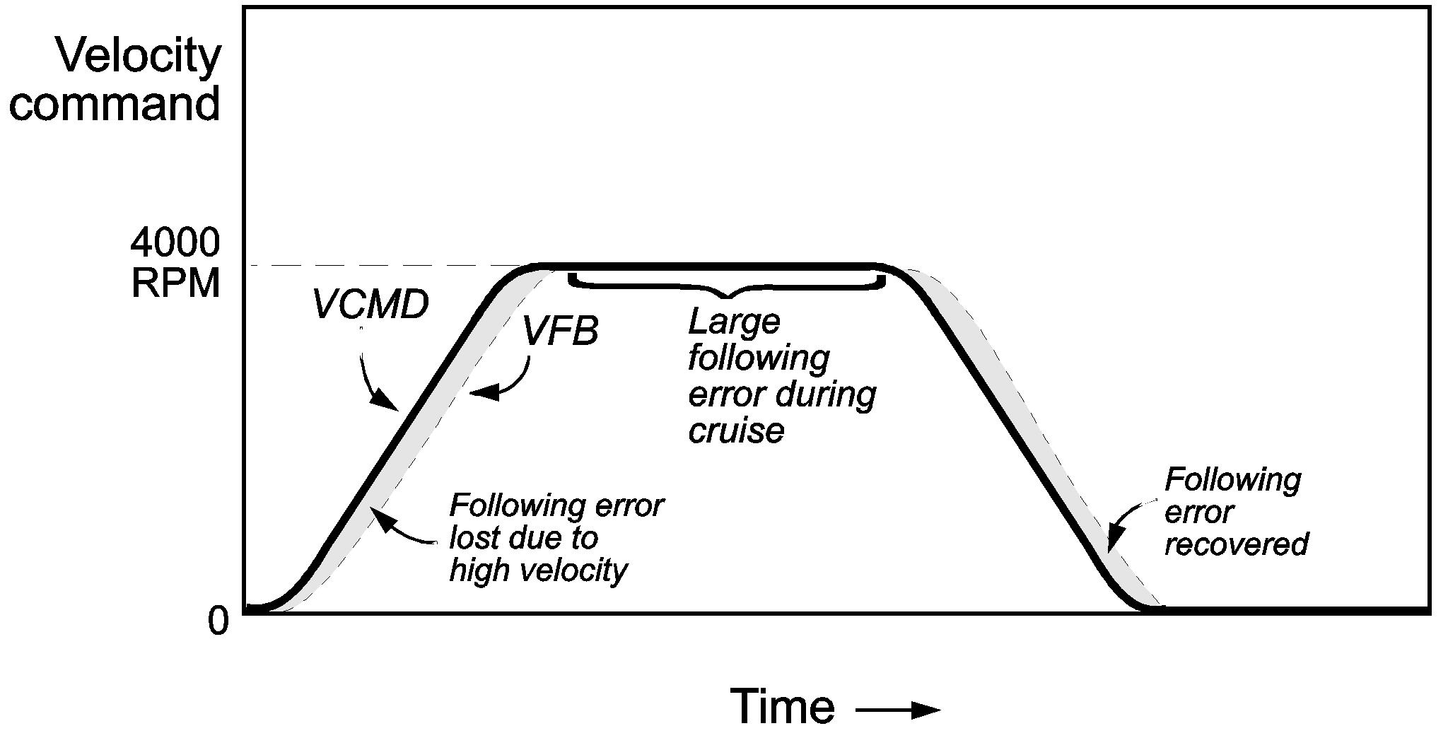
The proportional position loop is the simplest position loop. The velocity command is proportional to the following error. Large velocity commands need large following error limits. The constant of proportionality is GP (position loop gain). At first, this may seem confusing. Actually, it just means that for each count of position error, a command of GP RPM is given.The following error for acceleration with a typical proportional loop is shown below.

Reducing Position Error
Position error generated during a move is often called “following error” because it measures how well the motor follows the command. Reducing the following error is equivalent to following the command more closely, which normally is desirable. Commonly, you will set GP to be large, which reduces following error because the higher gain means it takes less position error to generate the same velocity command. There is a limit though, because if GP gets too large, the position loop becomes unstable. After GP is as large as possible, what else can you do to reduce position error?
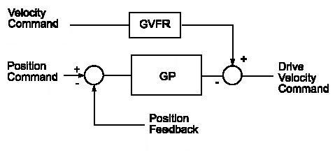
One technique to reduce following error is to add a feed-forward term to the velocity loop. This allows you to generate velocity commands with a combination of the profile velocity command and position error, rather than relying wholly on position error. A position loop with feed-forward is shown in the following figure.

In this case, you can reduce following error by raising the gain GVFR.
When GVFR is at full scale (GVFR =1), the following error at steady-state is reduced to zero. The only following error is generated during transients. The effect of full feed-forward on following error is shown in the following figure.

The benefit of full feed-forward is that it eliminates steady-state following error. The drawback is that the system overshoots when subjected to acceleration or deceleration. In some cases, this is not an issue because the system may always transition smoothly, or some overshoot may be acceptable. However, in many cases of full feed-forward is not acceptable. In these cases, you can reduce the feed-forward term to reduce overshoot. The larger the feed-forward gain, the greater reduction you will see in steady-state following error. Most systems can tolerate the overshoot generated by feed-forward gains of 50%.
OPMODE
This command allows you to change the drive operation mode.
Short form
None
Syntax
OpMode <value>
?OpMode'
Range
0 , 1 , 2 , 3 and 5 0 : Digital velocity opmode 1 : Analog velocity 2 : Digital torque 3 : Analog torque 5 : External position used as the digital position, the regular position mode
Units
NA
Default
5
Scope
Configuration, Task, Terminal
Limitations
Read/Write: R/W in CP4, Axis must be disabled.
Examples
OpModeOpMode 2
DIGITALTORQUE
Executes Digital Torque command ,similar to Jog command with automatic scaling of the profiler-velocity to torque. Automatically causes the SAC to enter digital torque mode. <Torque Value> Value of the target torque in mA, if greater then MICONT*100 then the later value will be used , sending a note to the user. TimeToTorque – time needed to reach the target torque value from the initial torque value . TimeTorque – duration of the torque command, if set to –1 (default) endless torque command. (Same as TimeJog) Type<Torque Value> : Double <TimeToTorque>: Long <TimeTorque>: - Long
Short form
DTorque
Syntax
DigitalTorque <Torque Value> {TimeToTorque=<time>} {<TimeTorque>=<time>} {<StartType=<starttype value>}
Range
- ±DIPEAK
Units
<Torque Value> : MilliAmperes
<TimeToTorque>: MSec
<TimeTorque>: MSec
Limitations
DigitalTorque OpMode.The axis must be attached to that task either implicitly (if no other task is accessing the axis) or explicitly using the “ATTACH” command.
Examples
DigitalTorque trq StartType=Immediate
TIMETOTORQUE
Defines the time needed to change the torque from an initial value to the value given in the DigitalTorque command.
Syntax
TimeToTorque=<time> DTorque <Torque Value> {TimeToTorque=<time>}
Type
Long
Range
1 to MaxLong
Units
Milliseconds
Scope
Task, Terminal
Limitations
Modal/Nodal .To set the value within a task, the axis must be attached to that task either implicitly (if no other task is accessing the axis) or explicitly using the “ATTACH” command.
Examples
?TimeToTorque
DigitalTorque 100 TimeToTorque = 1000
TIMETORQUE
Duration of the torque command .Time when the deceleration (torque decrease towards zero) is started, counting from the end of the torque increase. If set to –1 (default) endless torque command .
Syntax
DTorque <Torque Value> {TimeTorque=<time>}
Type
Long
Range
-1 , 0 to MaxLong
Units
Milliseconds
Default
1
Scope
Task, Terminal
Limitations
Nodal only.To set the value within a task, the axis must be attached to that task either implicitly (if no other task is accessing the axis) or explicitly using the “ATTACH” command.
Examples
DigitalTorque 100 TimeTorque = 1000