Difference between revisions of "Inverse Dynamic Model"
(→Identification process for different robot models) |
(→Identification process for different robot models) |
||
| Line 301: | Line 301: | ||
| − | + | Example for an identification task that will work for all types mentioned above: | |
| + | <syntaxhighlight lang='VB'> | ||
| + | 1. program | ||
| + | 2. dim startPoint as generic joint | ||
| + | 3. dim sineTarget as generic joint | ||
| + | 4. dim SWfreq as generic joint | ||
| + | 5. | ||
| + | 6. startPoint = -350 | ||
| + | 7. sineTarget = 350 | ||
| + | 8. SWfreq = 1.5 | ||
| + | 9. | ||
| + | 10. with axis | ||
| + | 11. attach | ||
| + | 11. En = 0 | ||
| + | 12. while En | ||
| + | 13. sleep 100 | ||
| + | 14. end while | ||
| + | 15. DynamicModel = 2 | ||
| + | 16. En = 1 | ||
| + | 17. while not En | ||
| + | 18. sleep 100 | ||
| + | 19. end while | ||
| + | 20. | ||
| + | 21. Move startPoint Abs = 1 | ||
| + | 22. while IsMoving | ||
| + | 23. sleep 100 | ||
| + | 24. end while | ||
| + | 25. | ||
| + | 26. SineWave sineTarget SineWaveFreq = SWfreq Abs = 1 | ||
| + | 27. sleep 2000 | ||
| + | 28. ' IdentFilterFreq is a Low pass filter.Frequency should be below 125 Hz | ||
| + | 29. IdentificationStart IdentFilterFreq = 80 | ||
| + | 30. ' the time of the identification, you can change time. | ||
| + | 31. sleep 20000 | ||
| + | 32. IdentificationFinish | ||
| + | 33. | ||
| + | 34. stop | ||
| + | 35. while IsMoving | ||
| + | 36. sleep 100 | ||
| + | 37. end while | ||
| + | 38. proceed | ||
| + | 39. En = 0 | ||
| + | 40. | ||
| + | 41. detach | ||
| + | 42. end with | ||
| + | 43. end program | ||
| + | |||
| + | </syntaxhighlight> | ||
| + | |||
| + | |||
| + | To reuse this code, remember to use frequency and amplitude values that are suited for the application, and also use the suitable dynamic model type. | ||
| − | |||
===SCARA robot=== | ===SCARA robot=== | ||
The SARA robot has two kinematic models, one with 3 axes (XYZ) and the other with four axes (XYZR). <br> | The SARA robot has two kinematic models, one with 3 axes (XYZ) and the other with four axes (XYZR). <br> | ||
Revision as of 14:02, 9 November 2017
Contents
- 1 Introduction - what is it good for and how does it work
- 2 Torque Units
- 3 How to perform the dynamic model parameters identification
- 4 Explanation of the identification output file
- 5 Explanation of the identification process recording file
- 6 Demonstration of tracking improvements (settling , position error)
- 7 Collision detection
- 8 Review of the possible reasons for an identification failure
- 9 How to assess what is the failure reason based on the output files
- 10 Test specifications
Introduction - what is it good for and how does it work
The inverse dynamic model (IDM) feature is used to compensate friction and dynamic effects for motion elements, otherwise leading to positioning errors and suboptimal settling and tracking behavior.
The motivation of the IDM feature is to use additional knowledge about the motion than just the position – i.e. velocity and torque – to offset the command values of the torque controller in order to make them react faster and thereby reduce the final positioning error and improve the settling behavior.
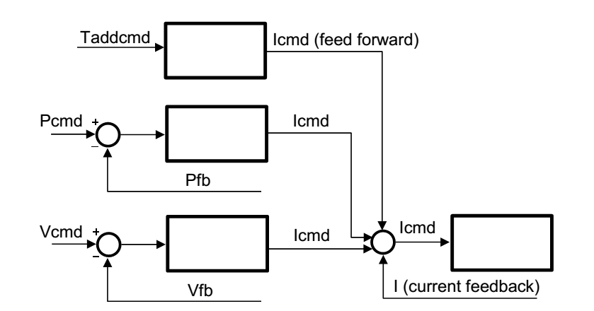
The term inverse dynamic model (often named computed torque control) means that the softMC takes a cartesian motion of a motion element and not only computes the joint position for the next Cartesian setpoint, but also the joint torque required for the motion. In order to be able to do that, it needs a dynamic model – i.e., a model of the masses and inertias – of the motion element. The joint velocity and torque are then sent to the drives as additional torque command data (see Figure 1).
In most cases, the user doesn’t have the parameters of the dynamic model. In such cases, those parameters can be estimated using the softMC identification process. The softMC allows to perform measurements and estimate the dynamic model parameters of some common robot models. The identification process is performed as follows: while the robot is commanded to perform a certain movement, the movement parameters and internal motors torques are recorded. Then, the dynamic model parameters of the robot are extracted based on the robot model and the measurements.
Torque Units
The MKS system of units defines the torque unit as [Nm] (Newton*meter). When dealing with motors, the torque is usually modeled as proportional to the current in the motors. Therefore, the torque can be defined with different units in each system. This section describes the torque units for each system and how they relate to each other.
The softMC reads the motor's torque through the drives, but not in [Nm] units. Therefore, the softMC contains an axis property called TorqueFactor (TFac) which divides the motor's torque parameter in order to convert it to desirable units. The result of this operation is stored in an axis property called TorqueFeedback.
CDHD Drive setup
The CDHD drives have the following parameters to define the motor's current properties:
- MICONT – in units of Ampere [A], but being read in units of milli-Ampere [mA], defines the motor continuous current. This is the maximum allowed value for long operation cycles.
- MIPEAK – in units of Ampere [A], but being read in units of milli-Ampere [mA], defines the motor peak current. This is the maximum allowed value for very short operation cycles.
- MKT – for rotary motors, being read in units of [Nm/A], defines the torque constant, i.e. how much torque the motor gives per Ampere unit.
- MKF – for linear motors, being read in units of [N/A], defines the force constant, i.e. how much force the motor gives per Ampere unit.
- I – being read in units of milli-MICONT [0.001*MICONT]. It indicates the actual value of the current. It corresponds to the current in the motor.
The TorqueFeedback property is calculated as follows:
Therefore, the TorqueFactor property should be set appropriately in order to convert the TorqueFeedback value to units of [Nm]:
The 1 million is in order to compensate for the MICONT being in units of [mA] and the Current Actual Value being in units of [0.001*MICONT]. Defining the TorqueFactor this way will convert the Current Actual Value to unit of [Nm] (and the value is assigned to TorqueFeedback). After setting Tfac, all values of torque (Tfb,TCmd,Tmax, TorqueThreshold, Te) will always be in units of [Nm] ([N] for linear axes). An example for this calculation in MC-Basic is presented in Figure 2.
EtherCAT and CANopen standart (DS402)
The EtherCAT standard defines the following parameters which are equivalent to the above parameters:
| CDHD parameter | EtherCAT parameter | EtherCat index |
|---|---|---|
| MICONT | Motor Rated Current | 0x6075 |
| MIPEAK | Motor Peak Current | 0x2036 |
| MKT | Torque Constant | 0x2039 |
| MKF | Torque Constant for Linear Motors | 0x2038 |
| I | Current Actual Value | 0x6078 |
The softMC has the following torque related properties:
- <axis>.TorqueThreshold - The axis torque threshold value is used to define the limit of the TADDCOMMAND value. If this value is exceeded, the softMC raises an error. One can set this value to some user desired value, or to a value matching the drive MICONT or MIPEAK values.
For example, setting the TorqueThreshold to a value that matches MICONT:
Setting the TorqueThreshold to a value that matches MIPEAK:
How to include gear ratio
Usually, the motors are connected to the joints through a gear system. The gear system affects the torque loads the motors carry and therefore the torque factors should be compensated appropriately. After this compensation, the TorqueFactor parameter transforms the Current Actual Value parameter from current inside the motors ([mMICONT] units) to the torques the joints are carrying (in [Nm] units).
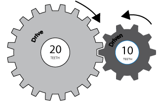
where GR stands for Gear Ratio. Figure 3 shows an example of a gear ratio.
Linear Axes
All of the above refers to rotary axes. Linear axes, in contrast to rotary axes, carry force and not torque. These forces are measured in units of Newton [N]. Therefore, some modifications should be made when dealing with Linear axes. Basically, there are two types of linear axes - Rotary motors with lead screws/pulleys/others, and Linear Motors.
Rotary motors with lead screws / pulleys / or different type of mechanism used to translate turning motion into linear motion
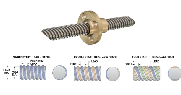
This type is treated the same as the regular rotary axes with a single modification. The mechanism used to translate turning motion into linear motion transforms the torque load, carried by the motor, to a force load on the linear axis. Therefore, the TorqueFactor should be multiplied by another factor. This parameter should contain the ratio between the amount of linear motion made per one rotation of the rotary motor (after the gear). For a lead screw, it would be the Screw Lead [mm/rev]. For a pulley, it would be the radius of the pulley multiplied by 2π [mm/rev]. The TorqueFactor would be:
When SL stands for Screw Lead or an equivalent parameter. figure 4 shows an example of a lead-screw lead.
Linear Motors
This type is treated the same as the regular rotary axes, but the MKT is switched with the MKF property, which is in units of [N/A] and there is no gear, therefore the TorqueFactor would be:
Operation Mode and PDOs
The operation mode of the drives while using the dynamic model should be cyclic synchronous position. The dynamic model is used to compute the required torque (or current) for each motor, however the results are never precise. The additive torque command is used only as a feed forward signal as mentioned in section 3.
Here is the list of additional PDOs (additional to the ‘cyclic synchronous position’ PDOs) that are necessary to use the dynamic model:
| PDO index | Description |
|---|---|
| RX: 0x60B2 | Torque Offset – the additive torque signal |
| TX 0x6078 | Current Actual Value – the torque feedback signal |
How to perform the dynamic model parameters identification
Data acquisition
The process of identification is done by moving the robot while recording the movement parameters and internal motors torques. Then, the recorded data is used to extract the dynamic model parameters based on the robot model and the measurements.
A good-quality data is important for obtaining good identification results. A high-quality data contains data points that are scattered over the movement space of the robot with varying velocities and accelerations. The scattered data yields a better fit of the parameters for a wide range of movements of the robot, allowing to predict the additive torque command with good accuracy.
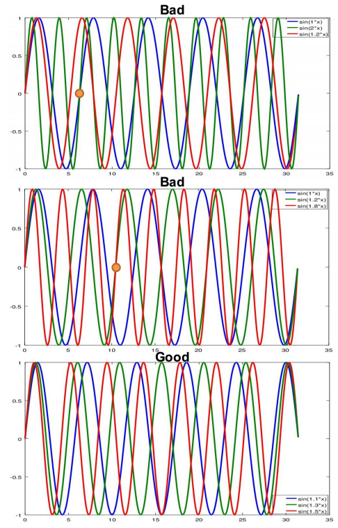
The recommended type of movement is using the sinewave command. This command moves each joint of the robot in a specified amplitude and frequency. In order to receive a good scattered data, the amplitude of each joint should be close to its full position range and the frequency of each joint should be different from the other joints. The frequency of each joint determined the correlation of movement between the joints. If two or more joints have the same frequency, they will always be in the same phase together and this will result in a non-scattered data. Furthermore, if the frequency of some joint is a multiplication of the frequency of another joint, the same motion will be repeated after a few cycles (more precisely, the factor of multiplication) of the faster joint. Actually, the motion will be repeated after a few cycles for any rational frequency values. However, in order to obtain good result, it is recommended to obtain data for at least three cycles for each joint. Therefore, as long as the motion does not repeat itself in this recorded time, the frequency selections is just fine. Here are some examples for a three joints robot:
| J1 | J2 | J3 | comment | Quality |
|---|---|---|---|---|
| 1 | 2 | 1.2 | j1 and j2 will repeat after 1 cycle o j1 and 2 cycles of j2 | Bad |
| 1 | 1.2 | 1.2 | j2 and j3 will repeat after 3 cycles of j2 and 2 cycles of j3 | Medium |
| 1.1 | 1.3 | 1.5 | j1, j2 and j3 will repeat after 11 cycles of j1, 13 cycles of j2 and 15 cycles of j3 | Good |
The first example is not a good choice of frequencies, the second example is fine, and the last example is a good choice of parameters. Graphs showing these combinations of sinewaves are presented in Figure 5.
Finally, the velocities of the joints are also important. The peak velocity during the motion should be close to the maximum velocity of each joint. In high velocities, the acceleration and velocity objects of the dynamic model are significant, thus allowing more accurate identification process. The peak velocities of the joints can be managed by the amplitude and frequency of the movement. It is more convenient to first define the amplitude of each joint, then set some arbitrary frequencies, for example {1.1,1.3,1.5}, and multiply the frequencies vector by a scalar factor: factor*{1.1,1.3,1.5}. By changing the factor, one can control the velocities of the joints.
Example of an identification task
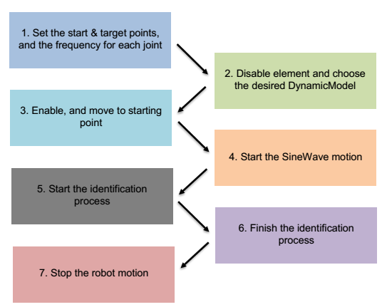
Figure 6 shows a schematic graph of the identification procedure.
Example of a program that executes the identification process, this program is for a delta robot:
1.  program
2.      dim startPoint as generic joint
3.      dim sineTarget as generic joint
4.      dim SWfreq as generic joint
5.
6.      startPoint = {-30,-30,-30,-200}
7.      sineTarget = {70,70,70,200}
8.      SWfreq = 0.3*{1,1.27,1.43,1.13}
9.
10.     with robot
11.         attach
11.	    En = 0
12.	    while En
13.	        sleep 100
14.	    end while
15.	    DynamicModel = 1
16.	    En = 1
17.	    while not En
18.	        sleep 100
19.	    end while
20.
21.	    Move startPoint Abs = 1
22.	    while IsMoving
23.	        sleep 100
24.	    end while
25.
26.	    SineWave sineTarget SineWaveFreq = SWfreq
27.	    sleep 2000
28.	' IdentFilterFreq is a Low pass filter.Frequency should be below 125 Hz
29.	    IdentificationStart IdentFilterFreq = 80
30.	' the time of the identification, you can change time.
31.	    sleep 20000
32.	    IdentificationFinish
33.
34.	    stop
35.	    while IsMoving
36.	        sleep 100
37.	    end while
38.	    proceed
39.	    En = 0
40.
41.	    detach
42.     end with
43. end program
Here is an explanation of the program shown:
| Line | Description | ||||||||||
|---|---|---|---|---|---|---|---|---|---|---|---|
| 6 | Defines the starting position of each joint of the system | ||||||||||
| 7 | Defines the ending position | ||||||||||
| 8 | Defines the frequency of the sinewave of each joint (note that the frequencies are multiplied by a factor of 0.3). Overall, these are the joints location in time:
| ||||||||||
| 15 | Defines the appropriate dynamic model of the robot, this will be discussed later on. Note, this parameter can be modified only when the robot is disabled. | ||||||||||
| 21 | Moves the robot to the starting position | ||||||||||
| 26 | Starts the sinewave movement with the target – sineTarget and freque ncy – SWfreq | ||||||||||
| 29 | starts the recording of the data with the IdentificationStart command. At this line, one can also set a low pass filter over the collected data (over pfb and tfb) with a cutoff frequency set to IdentFilterFreq. The cutoff frequency must be larger than the largest sinewave frequency. One can try several cutoff frequencies and compare between the raw and filtered data, then choose the one that filters most of the noise without changing the real data. Please look for the identification wiki page for more information regarding the parameters that could be set for IdentificationStart command | ||||||||||
| 31 | sets a sleeping time – the recording time | ||||||||||
| 32 | stops the recording and apply the dynamic model parameters identification |
At the end of this task, a files named IDNT<group num>.PRG and IDNT<group num>.REC will be created in the MC folder.
The PRG file contains the identified parameters and the REC file contains the recorded data used for the identification.
The following subsections explain how to apply the identification for different robot models.
Identification process for different robot models
Single axis model
There are two types of single axis joints, linear and rotary. Each of these types has several different dynamic models as can be viewed in the Dynamic Models wiki page (and in section 5.4). Here are the different models in short:
Linear axis
The linear axis type has 2 dynamic model types:
- Horizontal axis
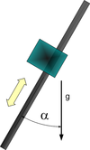
- Tilted axis – an axis with angle α relative to the vertical axis, ranging between 0 and 90 degrees (figure 7). When α = 0 the axis is vertical, and when α = 90 the axis is horizontal (the α parameter is found by the identification (i.e. it is not a user input).
Rotary axis
The rotary axis type has 3 dynamic model types:
- Simple rotary axis - which its center of mass is located on the rotation axis.
- Horizontal crank-arm axis (figure 8 left).
- Vertical crank-arm axis (figure 8 right).
Example for an identification task that will work for all types mentioned above:
1.  program
2.      dim startPoint as generic joint
3.      dim sineTarget as generic joint
4.      dim SWfreq as generic joint
5.
6.      startPoint = -350
7.      sineTarget = 350
8.      SWfreq = 1.5
9.
10.     with axis
11.         attach
11.	    En = 0
12.	    while En
13.	        sleep 100
14.	    end while
15.	    DynamicModel = 2
16.	    En = 1
17.	    while not En
18.	        sleep 100
19.	    end while
20.
21.	    Move startPoint Abs = 1
22.	    while IsMoving
23.	        sleep 100
24.	    end while
25.
26.	    SineWave sineTarget SineWaveFreq = SWfreq Abs = 1
27.	    sleep 2000
28.	' IdentFilterFreq is a Low pass filter.Frequency should be below 125 Hz
29.	    IdentificationStart IdentFilterFreq = 80
30.	' the time of the identification, you can change time.
31.	    sleep 20000
32.	    IdentificationFinish
33.
34.	    stop
35.	    while IsMoving
36.	        sleep 100
37.	    end while
38.	    proceed
39.	    En = 0
40.
41.	    detach
42.     end with
43. end program
To reuse this code, remember to use frequency and amplitude values that are suited for the application, and also use the suitable dynamic model type.
SCARA robot
The SARA robot has two kinematic models, one with 3 axes (XYZ) and the other with four axes (XYZR).
However, there is only one type of dynamic model which fits both of these kinematics models.
Example for an identification task that will work for 3 axes SCARA:
1.  program
2.      dim startPoint as generic joint
3.      dim sineTarget as generic joint
4.      dim SWfreq as generic joint
5.
6.      startPoint = {-160,-160,0}
7.      sineTarget = {160,160,150}
8.      SWfreq = 0.3*{1,1.27,1.43}
9.
10.     with SCARA
11.         attach
11.	    En = 0
12.	    while En
13.	        sleep 100
14.	    end while
15.	    DynamicModel = 1
16.	    En = 1
17.	    while not En
18.	        sleep 100
19.	    end while
20.
21.	    Move startPoint Abs = 1
22.	    while IsMoving
23.	        sleep 100
24.	    end while
25.
26.	    SineWave sineTarget SineWaveFreq = SWfreq
27.	    sleep 2000
28.	' IdentFilterFreq is a Low pass filter.Frequency should be below 125 Hz
29.	    IdentificationStart IdentFilterFreq = 80
30.	' the time of the identification, you can change time.
31.	    sleep 20000
32.	    IdentificationFinish
33.
34.	    stop
35.	    while IsMoving
36.	        sleep 100
37.	    end while
38.	    proceed
39.	    En = 0
40.
41.	    detach
42.     end with
43. end program
Example for an identification task that will work for 4 axes SCARA:
1.  program
2.      dim startPoint as generic joint
3.      dim sineTarget as generic joint
4.      dim SWfreq as generic joint
5.
6.      startPoint = {-160,-160,0,-350}
7.      sineTarget = {160,160,150,350}
8.      SWfreq = 0.3*{1,1.27,1.43,1.13}
9.
10.     with SCARA
11.         attach
11.	    En = 0
12.	    while En
13.	        sleep 100
14.	    end while
15.	    DynamicModel = 1
16.	    En = 1
17.	    while not En
18.	        sleep 100
19.	    end while
20.
21.	    Move startPoint Abs = 1
22.	    while IsMoving
23.	        sleep 100
24.	    end while
25.
26.	    SineWave sineTarget SineWaveFreq = SWfreq
27.	    sleep 2000
28.	' IdentFilterFreq is a Low pass filter.Frequency should be below 125 Hz
29.	    IdentificationStart IdentFilterFreq = 80
30.	' the time of the identification, you can change time.
31.	    sleep 20000
32.	    IdentificationFinish
33.
34.	    stop
35.	    while IsMoving
36.	        sleep 100
37.	    end while
38.	    proceed
39.	    En = 0
40.
41.	    detach
42.     end with
43. end program
To reuse this code, remember to use frequency and amplitude values that are suited for the application.
Some SCARA robots have coupled joints, usually the 3rd and 4th joints. Currently, the dynamic model of the SCARA robot does not take the coupling into account. Therefore, there may be large errors for coupled joints
DELTA robot
The Delta robot has two kinematic models, one with 3 axes (XYZ) and the other with four axes (XYZR).
However, there is only one type of dynamic model which fits both of these kinematics models.
Example for an identification task that will work for 3 axes Delta:
1.  program
2.      dim startPoint as generic joint
3.      dim sineTarget as generic joint
4.      dim SWfreq as generic joint
5.
6.      startPoint = {-30,-30,-30}
7.      sineTarget = {70,70,70}
8.      SWfreq = 0.3*{1,1.27,1.43}
9.
10.     with DELTA
11.         attach
11.	    En = 0
12.	    while En
13.	        sleep 100
14.	    end while
15.	    DynamicModel = 1
16.	    En = 1
17.	    while not En
18.	        sleep 100
19.	    end while
20.
21.	    Move startPoint Abs = 1
22.	    while IsMoving
23.	        sleep 100
24.	    end while
25.
26.	    SineWave sineTarget SineWaveFreq = SWfreq
27.	    sleep 2000
28.	' IdentFilterFreq is a Low pass filter.Frequency should be below 125 Hz
29.	    IdentificationStart IdentFilterFreq = 80
30.	' the time of the identification, you can change time.
31.	    sleep 20000
32.	    IdentificationFinish
33.
34.	    stop
35.	    while IsMoving
36.	        sleep 100
37.	    end while
38.	    proceed
39.	    En = 0
40.
41.	    detach
42.     end with
43. end program
Example for an identification task that will work for 4 axes Delta:
1.  program
2.      dim startPoint as generic joint
3.      dim sineTarget as generic joint
4.      dim SWfreq as generic joint
5.
6.      startPoint = {-30,-30,-30,-350}
7.      sineTarget = {70,70,70,350}
8.      SWfreq = 0.3*{1,1.27,1.43,1.13}
9.
10.     with DELTA
11.         attach
11.	    En = 0
12.	    while En
13.	        sleep 100
14.	    end while
15.	    DynamicModel = 1
16.	    En = 1
17.	    while not En
18.	        sleep 100
19.	    end while
20.
21.	    Move startPoint Abs = 1
22.	    while IsMoving
23.	        sleep 100
24.	    end while
25.
26.	    SineWave sineTarget SineWaveFreq = SWfreq
27.	    sleep 2000
28.	' IdentFilterFreq is a Low pass filter.Frequency should be below 125 Hz
29.	    IdentificationStart IdentFilterFreq = 80
30.	' the time of the identification, you can change time.
31.	    sleep 20000
32.	    IdentificationFinish
33.
34.	    stop
35.	    while IsMoving
36.	        sleep 100
37.	    end while
38.	    proceed
39.	    En = 0
40.
41.	    detach
42.     end with
43. end program
To reuse this code, remember to use frequency and amplitude values that are suited for the application.
PUMA robot
The PUMA robot has only one kinematic model but it has two different dynamic models.
The first dynamic model is a regular model like the other robots.
The second model is a semi-static model, meaning it will work only for slow movements and static positions. This model takes into account only the gravity and friction forces / torques.
Full regular model
This model identification rules are just like the previous models.
Example for an identification task that will work for PUMA:
1.  program
2.      dim startPoint as generic joint
3.      dim sineTarget as generic joint
4.      dim SWfreq as generic joint
5.
6.      startPoint = {-100,-170,100,-60,-60,-100}
7.      sineTarget = {100,-40,235,60,60,100}
8.      SWfreq = 0.15*{1.56,1,1.31,1.47,1.21,1.17}
9.
10.     with PUMA
11.         attach
11.	    En = 0
12.	    while En
13.	        sleep 100
14.	    end while
15.	    DynamicModel = 1
16.	    En = 1
17.	    while not En
18.	        sleep 100
19.	    end while
20.
21.	    Move startPoint Abs = 1
22.	    while IsMoving
23.	        sleep 100
24.	    end while
25.
26.	    SineWave sineTarget SineWaveFreq = SWfreq
27.	    sleep 2000
28.	' IdentFilterFreq is a Low pass filter.Frequency should be below 125 Hz
29.	    IdentificationStart IdentFilterFreq = 80
30.	' the time of the identification, you can change time.
31.	    sleep 20000
32.	    IdentificationFinish
33.
34.	    stop
35.	    while IsMoving
36.	        sleep 100
37.	    end while
38.	    proceed
39.	    En = 0
40.
41.	    detach
42.     end with
43. end program
To reuse this code, remember to use frequency and amplitude values that are suited for the application.
Semi-static model
The semi-static model identification is a little bit different from all of the examples so far. This model takes into account only gravity and friction forces, in other words it neglects dynamic forces. Therefore, the measurement should include negligible dynamic forces, and this is possible by moving slow.
This identification process is longer than the usual identification progress, it takes approximately 2-3 minutes. In addition, it is advised to perform less than 3 cycles, 1 cycle should be enough.
Also, similar to the previous examples, the semi-static model threshold the velocity of the data points. But unlike the previous examples, here there are two thresholds, one for avoiding very low velocities avoiding numeric errors) and the other for avoiding high velocities (avoiding significant dynamic forces).
Example for such an identification process:
1.  program
2.      dim startPoint as generic joint
3.      dim sineTarget as generic joint
4.      dim SWfreq as generic joint
5.
6.      startPoint = {-100,-170,100,-60,-60,-100}
7.      sineTarget = {100,-40,235,60,60,100}
8.      SWfreq = 0.02*{1.56,1,1.31,1.47,1.21,1.17}
9.
10.     with PUMA
11.         attach
11.	    En = 0
12.	    while En
13.	        sleep 100
14.	    end while
15.	    DynamicModel = 1
16.	    En = 1
17.	    while not En
18.	        sleep 100
19.	    end while
20.
21.	    Move startPoint Abs = 1
22.	    while IsMoving
23.	        sleep 100
24.	    end while
25.
26.	    SineWave sineTarget SineWaveFreq = SWfreq
27.	    sleep 2000
28.	' IdentFilterFreq is a Low pass filter.Frequency should be below 125 Hz
29.	    IdentificationStart IdentFilterFreq = 80
30.	' the time of the identification, you can change time.
31.	    sleep 20000
32.	    IdentificationFinish
33.
34.	    stop
35.	    while IsMoving
36.	        sleep 100
37.	    end while
38.	    proceed
39.	    En = 0
40.
41.	    detach
42.     end with
43. end program
Note the significant low frequencies which cause slow movement.
