Difference between revisions of "Inverse Dynamic Model"
(Added comment about Direction.) |
|||
| (10 intermediate revisions by 3 users not shown) | |||
| Line 1: | Line 1: | ||
| − | {{Languages}} | + | {{Languages|Inverse_Dynamic_Model}} |
<div id="BackToTop" class="noprint" style="background-color:; position:fixed; bottom:32px; left:95%; z-index:9999; padding:0; margin:0;"> | <div id="BackToTop" class="noprint" style="background-color:; position:fixed; bottom:32px; left:95%; z-index:9999; padding:0; margin:0;"> | ||
<span style="color:blue; font-size:8pt; font-face:verdana,sans-serif; border:0.2em outset:#ceebf7; padding:0.1em; font-weight:bolder; -moz-border-radius:8px; "> | <span style="color:blue; font-size:8pt; font-face:verdana,sans-serif; border:0.2em outset:#ceebf7; padding:0.1em; font-weight:bolder; -moz-border-radius:8px; "> | ||
| Line 29: | Line 29: | ||
The softMC reads the motor's torque through the drives, but not in [Nm] units. Therefore, the softMC contains an axis property called TorqueFactor (TFac) which divides the motor's torque parameter in order to convert it to desirable units. The result of this operation is stored in an axis property called [[MC-Basic:element.TORQUEFEEDBACK| TorqueFeedback]]. | The softMC reads the motor's torque through the drives, but not in [Nm] units. Therefore, the softMC contains an axis property called TorqueFactor (TFac) which divides the motor's torque parameter in order to convert it to desirable units. The result of this operation is stored in an axis property called [[MC-Basic:element.TORQUEFEEDBACK| TorqueFeedback]]. | ||
| − | |||
| − | |||
| − | |||
| − | |||
| − | |||
| − | |||
| − | |||
| − | + | == CDHD Drive setup == | |
| − | |||
| − | + | The CDHD drives have the following parameters to define the motor's current properties: | |
| − | |||
| + | *'''MICONT''' – in units of Ampere [A], but being read in units of milli-Ampere [mA], defines the motor continuous current. This is the maximum allowed value for long operation cycles. | ||
| + | *'''MIPEAK''' – in units of Ampere [A], but being read in units of milli-Ampere [mA], defines the motor peak current. This is the maximum allowed value for very short operation cycles. | ||
| + | *'''MKT''' – for rotary motors, being read in units of [Nm/A], defines the torque constant, i.e. how much torque the motor gives per Ampere unit. | ||
| + | *'''MKF''' – for linear motors, being read in units of [N/A], defines the force constant, i.e. how much force the motor gives per Ampere unit. | ||
| + | *'''I''' – being read in units of milli-MICONT [0.001*MICONT]. It indicates the actual value of the current. It corresponds to the current in the motor. | ||
| + | The TorqueFeedback property is calculated as follows: | ||
| + | <center><math>TFb = \frac{Current Actual Value}{Tfac}\ </math></center> | ||
| + | Therefore, the TorqueFactor property should be set appropriately in order to convert the TorqueFeedback value to units of [Nm]: | ||
| + | <center><math>TFac = \frac{Direction*1000000}{MKT*MICONT}\ </math></center> | ||
The 1 million is in order to compensate for the MICONT being in units of [mA] and the Current Actual Value being in units of [0.001*MICONT]. Defining the TorqueFactor this way will convert the Current Actual Value to unit of [Nm] (and the value is assigned to TorqueFeedback). After setting Tfac, all values of torque (Tfb,TCmd,Tmax, TorqueThreshold, Te) will always be in units of [Nm] ([N] for linear axes). An example for this calculation in MC-Basic is presented in Figure 2. | The 1 million is in order to compensate for the MICONT being in units of [mA] and the Current Actual Value being in units of [0.001*MICONT]. Defining the TorqueFactor this way will convert the Current Actual Value to unit of [Nm] (and the value is assigned to TorqueFeedback). After setting Tfac, all values of torque (Tfb,TCmd,Tmax, TorqueThreshold, Te) will always be in units of [Nm] ([N] for linear axes). An example for this calculation in MC-Basic is presented in Figure 2. | ||
| + | |||
| + | Note that the axis direction, especially in robots, must comply with the definitions of the [[Dynamic_Models|dynamic models]]. Since the actual positive motor direction might be in the oposite direction, the axis property [[MC-Basic:axis.DIRECTION|Direction]] must be used in order to correct it by software. The TorqueFactor must include Direction in order for the torque sign to agree with the motion direction. | ||
==EtherCAT and CANopen standart (DS402)== | ==EtherCAT and CANopen standart (DS402)== | ||
| Line 80: | Line 82: | ||
The softMC has the following torque related properties: | The softMC has the following torque related properties: | ||
| − | * '''''<axis>''.TorqueThreshold''' | + | |
| − | For example, setting the TorqueThreshold to a value that matches MICONT: <br> | + | * '''''<axis>''.TorqueMax'''<br> |
| + | * '''''<axis>''.TorqueThreshold'''<br> | ||
| + | |||
| + | These parameters are used to define the limit of the '''TADDCOMMAND''' value.<br> | ||
| + | The difference between those parameters is that '''TorqueMax''' is taken into account when the motion is being planned and '''TorqueThreshold''' limits the torque feedback. <br> | ||
| + | For example, if the planned motion exceeds TorqueMax, then an error will be thrown before the motion has started. However, if the planned motion is O.K, and the axis/robot started the motion, if the torque feedback crosses the TorqueThreshold, the robot motion will be stopped and an error will be thrown. <br> | ||
| + | One can set these parameters to some user desired value, or to a value matching the drive MICONT or MIPEAK values. <br> | ||
| + | |||
| + | For example, setting the TorqueThreshold to a value that matches '''MICONT''': <br> | ||
<center> <math> <axis>.TorqueThreshold = \frac{1000}{TFac}\ </math> </center> | <center> <math> <axis>.TorqueThreshold = \frac{1000}{TFac}\ </math> </center> | ||
| Line 89: | Line 99: | ||
* '''''<axis>''.AdditiveTorqueDelay''' - The calculated additive torque command is based on ''pcmd'' and ''vcmd''. Since there is a delay between the commands and the actual position and velocity of the axis, the same delay should be presented to the additive torque. The '''AdditiveTorqueDelay''' is used for this purpose. This property is in units of cycle time and it accepts positive integer values. The '''AdditiveTorqueDelay''' works as follows: the calculated additive torque command for a certain time would be sent to the drives only “AdditiveTorqueDelay” steps later. The default value of this property is 3. | * '''''<axis>''.AdditiveTorqueDelay''' - The calculated additive torque command is based on ''pcmd'' and ''vcmd''. Since there is a delay between the commands and the actual position and velocity of the axis, the same delay should be presented to the additive torque. The '''AdditiveTorqueDelay''' is used for this purpose. This property is in units of cycle time and it accepts positive integer values. The '''AdditiveTorqueDelay''' works as follows: the calculated additive torque command for a certain time would be sent to the drives only “AdditiveTorqueDelay” steps later. The default value of this property is 3. | ||
| − | ==How to include gear ratio== | + | |
| + | == How to include gear ratio == | ||
Usually, the motors are connected to the joints through a gear system. The gear system affects the torque loads the motors carry and therefore the torque factors should be compensated appropriately. After this compensation, the TorqueFactor parameter transforms the Current Actual Value parameter from current inside the motors ([mMICONT] units) to the torques the joints are carrying (in [Nm] units). | Usually, the motors are connected to the joints through a gear system. The gear system affects the torque loads the motors carry and therefore the torque factors should be compensated appropriately. After this compensation, the TorqueFactor parameter transforms the Current Actual Value parameter from current inside the motors ([mMICONT] units) to the torques the joints are carrying (in [Nm] units). | ||
| − | <center> <math> TFac = \frac{1000000}{MKT*MICONT*GR}\ </math></center> | + | <center><math>TFac = \frac{Direction*1000000}{MKT*MICONT*GR}\ </math></center> |
| − | |||
where GR stands for Gear Ratio. Figure 3 shows an example of a gear ratio. | where GR stands for Gear Ratio. Figure 3 shows an example of a gear ratio. | ||
| − | [[ | + | [[File:DM 2.png|frame|left|80px|<big><center>''figure 2 - Setting the torque factor(TFac) property for all axes in MC-Basic for WtherCAT drive''</center></big>]] |
| + | [[File:DM 3.png|frame|left|150px|<big><center>''figure 3 - An example of a gear mechanism with a ratio of 1:2''</center></big>]] | ||
| − | |||
==Linear Axes== | ==Linear Axes== | ||
All of the above refers to rotary axes. Linear axes, in contrast to rotary axes, carry force and not torque. These forces are measured in units of Newton [N]. Therefore, some modifications should be made when dealing with Linear axes. Basically, there are two types of linear axes - Rotary motors with lead screws/pulleys/others, and Linear Motors. | All of the above refers to rotary axes. Linear axes, in contrast to rotary axes, carry force and not torque. These forces are measured in units of Newton [N]. Therefore, some modifications should be made when dealing with Linear axes. Basically, there are two types of linear axes - Rotary motors with lead screws/pulleys/others, and Linear Motors. | ||
| − | |||
| − | |||
| − | |||
| − | |||
| − | + | === Rotary motors with lead screws / pulleys / or different type of mechanism used to translate turning motion into linear motion === | |
| − | + | This type is treated the same as the regular rotary axes with a single modification. The mechanism used to translate turning motion into linear motion transforms the torque load, carried by the motor, to a force load on the linear axis. Therefore, the TorqueFactor should be multiplied by another factor. This parameter should contain the ratio between the amount of linear motion made per one rotation of the rotary motor (after the gear). For a lead screw, it would be the Screw Lead [mm/rev]. For a pulley, it would be the radius of the pulley multiplied by 2π [mm/rev]. The TorqueFactor would be: | |
| − | [[ | + | <center><math>TFac = \frac{Direction*1000000*SL}{MKT*MICONT*GR*\pi} </math></center> |
| + | Where '''SL''' stands for Screw Lead or an equivalent parameter. figure 4 shows an example of a lead-screw lead.<br/> '''NOTE:''' '''SL''' is in units of [m/rev] -> meters per revolution. | ||
| + | [[File:DM 4.png|frame|center|300px|<big><center>''figure 4 - An example of a lead-screw (top) and a lead-screw lead (bottom)''</center></big>]] | ||
| − | ===Linear Motors=== | + | === Linear Motors === |
| − | |||
| − | |||
| + | This type is treated the same as the regular rotary axes, but the '''MKT''' is switched with the '''MKF''' property, which is in units of [N/A] and there is no gear, therefore the TorqueFactor would be: | ||
| + | <center><math>TFac = \frac{Direction*1000000}{MKF*MICONT}\ </math></center> | ||
===Operation Mode and PDOs=== | ===Operation Mode and PDOs=== | ||
| Line 295: | Line 303: | ||
===Single axis model=== | ===Single axis model=== | ||
There are two types of single axis joints, linear and rotary. Each of these types has several different dynamic models as can be viewed in the Dynamic Models wiki page (and in section 5.4). Here are the different models in short: | There are two types of single axis joints, linear and rotary. Each of these types has several different dynamic models as can be viewed in the Dynamic Models wiki page (and in section 5.4). Here are the different models in short: | ||
| − | ====Linear axis==== | + | |
| − | The linear axis type has | + | ==== Linear axis ==== |
| − | # Horizontal axis | + | |
| − | # Tilted axis – an axis with angle α relative to the vertical axis, ranging between 0 and 90 degrees (figure 7). When α = 0 the axis is vertical, and when α = 90 the axis is horizontal (the α parameter is found by the identification (i.e. it is not a user input). [[ | + | The linear axis type has 3 dynamic model types: |
| + | |||
| + | #Horizontal axis | ||
| + | #Tilted axis – an axis with angle α relative to the vertical axis, ranging between 0 and 90 degrees (figure 7). When α = 0 the axis is vertical, and when α = 90 the axis is horizontal (the α parameter is found by the identification (i.e. it is not a user input). | ||
| + | #Vertical axis with a spring.[[File:DM 8.png|thumb|right|200px|<center><big>''figure 7 - tilted linear axis''</big></center>]] | ||
====Rotary axis==== | ====Rotary axis==== | ||
Latest revision as of 05:40, 19 October 2025
| Language: | English • 中文(简体) |
|---|
Contents
- 1 Introduction - what is it good for and how does it work
- 2 Torque Units
- 3 How to perform the dynamic model parameters identification
- 4 Explanation of the identification output file
- 5 Explanation of the identification process recording file
- 6 Demonstration of tracking improvements (settling, position error)
- 7 Collision detection
- 8 Review of the possible reasons for an identification failure
- 9 How to assess what is the failure reason based on the output files
- 10 Test specifications
Introduction - what is it good for and how does it work
The inverse dynamic model (IDM) feature is used to compensate friction and dynamic effects for motion elements, otherwise leading to positioning errors and suboptimal settling and tracking behavior.
The motivation of the IDM feature is to use additional knowledge about the motion than just the position – i.e. velocity and torque – to offset the command values of the torque controller in order to make them react faster and thereby reduce the final positioning error and improve the settling behavior.
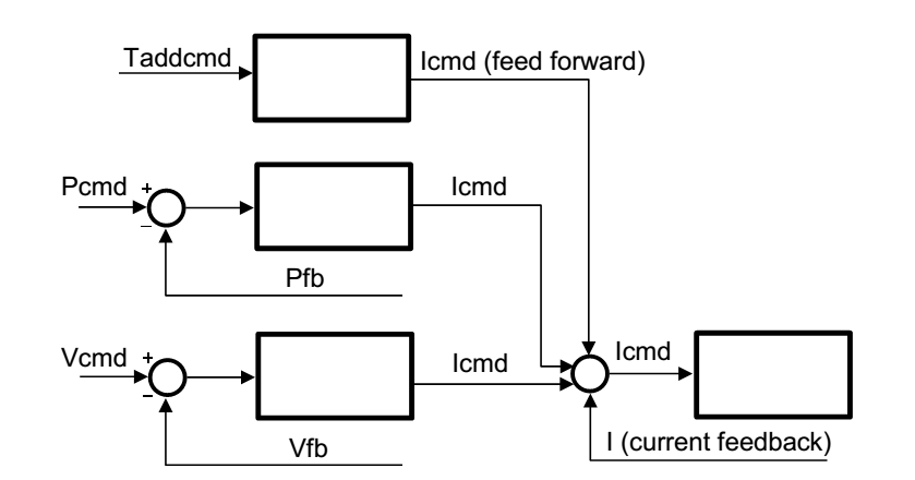
The term inverse dynamic model (often named computed torque control) means that the softMC takes a cartesian motion of a motion element and not only computes the joint position for the next Cartesian setpoint, but also the joint torque required for the motion. In order to be able to do that, it needs a dynamic model – i.e., a model of the masses and inertias – of the motion element. The joint velocity and torque are then sent to the drives as additional torque command data (see Figure 1).
In most cases, the user doesn’t have the parameters of the dynamic model. In such cases, those parameters can be estimated using the softMC identification process. The softMC allows to perform measurements and estimate the dynamic model parameters of some common robot models. The identification process is performed as follows: while the robot is commanded to perform a certain movement, the movement parameters and internal motors torques are recorded. Then, the dynamic model parameters of the robot are extracted based on the robot model and the measurements.
Torque Units
The MKS system of units defines the torque unit as [Nm] (Newton*meter). When dealing with motors, the torque is usually modeled as proportional to the current in the motors. Therefore, the torque can be defined with different units in each system. This section describes the torque units for each system and how they relate to each other.
The softMC reads the motor's torque through the drives, but not in [Nm] units. Therefore, the softMC contains an axis property called TorqueFactor (TFac) which divides the motor's torque parameter in order to convert it to desirable units. The result of this operation is stored in an axis property called TorqueFeedback.
CDHD Drive setup
The CDHD drives have the following parameters to define the motor's current properties:
- MICONT – in units of Ampere [A], but being read in units of milli-Ampere [mA], defines the motor continuous current. This is the maximum allowed value for long operation cycles.
- MIPEAK – in units of Ampere [A], but being read in units of milli-Ampere [mA], defines the motor peak current. This is the maximum allowed value for very short operation cycles.
- MKT – for rotary motors, being read in units of [Nm/A], defines the torque constant, i.e. how much torque the motor gives per Ampere unit.
- MKF – for linear motors, being read in units of [N/A], defines the force constant, i.e. how much force the motor gives per Ampere unit.
- I – being read in units of milli-MICONT [0.001*MICONT]. It indicates the actual value of the current. It corresponds to the current in the motor.
The TorqueFeedback property is calculated as follows:
Therefore, the TorqueFactor property should be set appropriately in order to convert the TorqueFeedback value to units of [Nm]:
The 1 million is in order to compensate for the MICONT being in units of [mA] and the Current Actual Value being in units of [0.001*MICONT]. Defining the TorqueFactor this way will convert the Current Actual Value to unit of [Nm] (and the value is assigned to TorqueFeedback). After setting Tfac, all values of torque (Tfb,TCmd,Tmax, TorqueThreshold, Te) will always be in units of [Nm] ([N] for linear axes). An example for this calculation in MC-Basic is presented in Figure 2.
Note that the axis direction, especially in robots, must comply with the definitions of the dynamic models. Since the actual positive motor direction might be in the oposite direction, the axis property Direction must be used in order to correct it by software. The TorqueFactor must include Direction in order for the torque sign to agree with the motion direction.
EtherCAT and CANopen standart (DS402)
The EtherCAT standard defines the following parameters which are equivalent to the above parameters:
| CDHD parameter | EtherCAT parameter | EtherCat index |
|---|---|---|
| MICONT | Motor Rated Current | 0x6075 |
| MIPEAK | Motor Peak Current | 0x2036 |
| MKT | Torque Constant | 0x2039 |
| MKF | Torque Constant for Linear Motors | 0x2038 |
| I | Current Actual Value | 0x6078 |
The softMC has the following torque related properties:
- <axis>.TorqueMax
- <axis>.TorqueThreshold
These parameters are used to define the limit of the TADDCOMMAND value.
The difference between those parameters is that TorqueMax is taken into account when the motion is being planned and TorqueThreshold limits the torque feedback.
For example, if the planned motion exceeds TorqueMax, then an error will be thrown before the motion has started. However, if the planned motion is O.K, and the axis/robot started the motion, if the torque feedback crosses the TorqueThreshold, the robot motion will be stopped and an error will be thrown.
One can set these parameters to some user desired value, or to a value matching the drive MICONT or MIPEAK values.
For example, setting the TorqueThreshold to a value that matches MICONT:
Setting the TorqueThreshold to a value that matches MIPEAK:
- <axis>.AdditiveTorqueDelay - The calculated additive torque command is based on pcmd and vcmd. Since there is a delay between the commands and the actual position and velocity of the axis, the same delay should be presented to the additive torque. The AdditiveTorqueDelay is used for this purpose. This property is in units of cycle time and it accepts positive integer values. The AdditiveTorqueDelay works as follows: the calculated additive torque command for a certain time would be sent to the drives only “AdditiveTorqueDelay” steps later. The default value of this property is 3.
How to include gear ratio
Usually, the motors are connected to the joints through a gear system. The gear system affects the torque loads the motors carry and therefore the torque factors should be compensated appropriately. After this compensation, the TorqueFactor parameter transforms the Current Actual Value parameter from current inside the motors ([mMICONT] units) to the torques the joints are carrying (in [Nm] units).
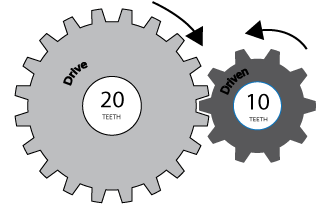
where GR stands for Gear Ratio. Figure 3 shows an example of a gear ratio.
Linear Axes
All of the above refers to rotary axes. Linear axes, in contrast to rotary axes, carry force and not torque. These forces are measured in units of Newton [N]. Therefore, some modifications should be made when dealing with Linear axes. Basically, there are two types of linear axes - Rotary motors with lead screws/pulleys/others, and Linear Motors.
Rotary motors with lead screws / pulleys / or different type of mechanism used to translate turning motion into linear motion
This type is treated the same as the regular rotary axes with a single modification. The mechanism used to translate turning motion into linear motion transforms the torque load, carried by the motor, to a force load on the linear axis. Therefore, the TorqueFactor should be multiplied by another factor. This parameter should contain the ratio between the amount of linear motion made per one rotation of the rotary motor (after the gear). For a lead screw, it would be the Screw Lead [mm/rev]. For a pulley, it would be the radius of the pulley multiplied by 2π [mm/rev]. The TorqueFactor would be:
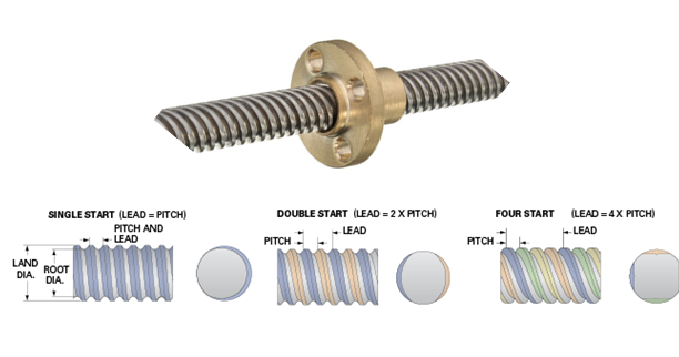
Where SL stands for Screw Lead or an equivalent parameter. figure 4 shows an example of a lead-screw lead.
NOTE: SL is in units of [m/rev] -> meters per revolution.
Linear Motors
This type is treated the same as the regular rotary axes, but the MKT is switched with the MKF property, which is in units of [N/A] and there is no gear, therefore the TorqueFactor would be:
Operation Mode and PDOs
The operation mode of the drives while using the dynamic model should be cyclic synchronous position. The dynamic model is used to compute the required torque (or current) for each motor, however the results are never precise. The additive torque command is used only as a feed forward signal as mentioned in section 3.
Here is the list of additional PDOs (additional to the ‘cyclic synchronous position’ PDOs) that are necessary to use the dynamic model:
| PDO index | Description |
|---|---|
| RX: 0x60B2 | Torque Offset – the additive torque signal |
| TX 0x6078 | Current Actual Value – the torque feedback signal |
How to perform the dynamic model parameters identification
Data acquisition
The process of identification is done by moving the robot while recording the movement parameters and internal motors torques. Then, the recorded data is used to extract the dynamic model parameters based on the robot model and the measurements.
A good-quality data is important for obtaining good identification results. A high-quality data contains data points that are scattered over the movement space of the robot with varying velocities and accelerations. The scattered data yields a better fit of the parameters for a wide range of movements of the robot, allowing to predict the additive torque command with good accuracy.
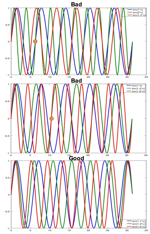
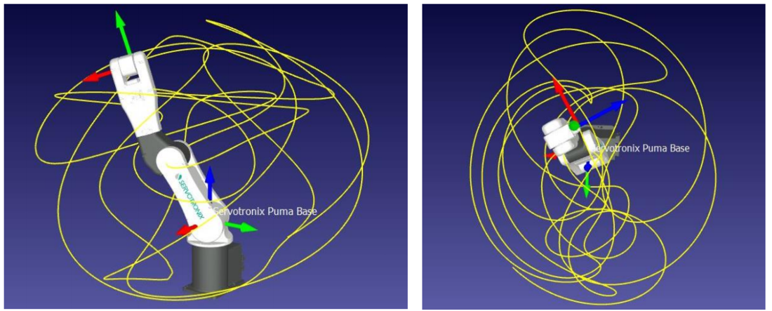
The recommended type of movement is using the sinewave command. This command moves each joint of the robot in a specified amplitude and frequency. In order to receive a good scattered data, the amplitude of each joint should be close to its full position range and the frequency of each joint should be different from the other joints. The frequency of each joint determined the correlation of movement between the joints. If two or more joints have the same frequency, they will always be in the same phase together and this will result in a non-scattered data. Furthermore, if the frequency of some joint is a multiplication of the frequency of another joint, the same motion will be repeated after a few cycles (more precisely, the factor of multiplication) of the faster joint. Actually, the motion will be repeated after a few cycles for any rational frequency values. However, in order to obtain good result, it is recommended to obtain data for at least three cycles for each joint. Therefore, as long as the motion does not repeat itself in this recorded time, the frequency selections is just fine. Here are some examples for a three joints robot:
| J1 | J2 | J3 | comment | Quality |
|---|---|---|---|---|
| 1 | 2 | 1.2 | j1 and j2 will repeat after 1 cycle o j1 and 2 cycles of j2 | Bad |
| 1 | 1.2 | 1.2 | j2 and j3 will repeat after 3 cycles of j2 and 2 cycles of j3 | Medium |
| 1.1 | 1.3 | 1.5 | j1, j2 and j3 will repeat after 11 cycles of j1, 13 cycles of j2 and 15 cycles of j3 | Good |
The first example is not a good choice of frequencies, the second example is fine, and the last example is a good choice of parameters. Graphs showing these combinations of sinewaves are presented in Figure 5.
Finally, the velocities of the joints are also important. The peak velocity during the motion should be close to the maximum velocity of each joint. In high velocities, the acceleration and velocity objects of the dynamic model are significant, thus allowing more accurate identification process. The peak velocities of the joints can be managed by the amplitude and frequency of the movement. It is more convenient to first define the amplitude of each joint, then set some arbitrary frequencies, for example {1.1,1.3,1.5}, and multiply the frequencies vector by a scalar factor: factor*{1.1,1.3,1.5}. By changing the factor, one can control the velocities of the joints.
Example of an identification task
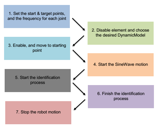
Figure 6 shows a schematic graph of the identification procedure.
Example of a program that executes the identification process, this program is for a delta robot:
1.  program
2.      dim startPoint as generic joint
3.      dim sineTarget as generic joint
4.      dim SWfreq as generic joint
5.
6.      startPoint = {-30,-30,-30,-200}
7.      sineTarget = {70,70,70,200}
8.      SWfreq = 0.3*{1,1.27,1.43,1.13}
9.
10.     with robot
11.         attach
11.	    En = 0
12.	    while En
13.	        sleep 100
14.	    end while
15.	    DynamicModel = 1
16.	    En = 1
17.	    while not En
18.	        sleep 100
19.	    end while
20.
21.	    Move startPoint Abs = 1
22.	    while IsMoving
23.	        sleep 100
24.	    end while
25.
26.	    SineWave sineTarget SineWaveFreq = SWfreq
27.	    sleep 2000
28.	' IdentFilterFreq is a Low pass filter.Frequency should be below 125 Hz
29.	    IdentificationStart IdentFilterFreq = 80
30.	' the time of the identification, you can change time.
31.	    sleep 20000
32.	    IdentificationFinish
33.
34.	    stop
35.	    while IsMoving
36.	        sleep 100
37.	    end while
38.	    proceed
39.	    En = 0
40.
41.	    detach
42.     end with
43. end program
Here is an explanation of the program shown:
| Line | Description | ||||||||||
|---|---|---|---|---|---|---|---|---|---|---|---|
| 6 | Defines the starting position of each joint of the system | ||||||||||
| 7 | Defines the ending position | ||||||||||
| 8 | Defines the frequency of the sinewave of each joint (note that the frequencies are multiplied by a factor of 0.3). Overall, these are the joints location in time:
| ||||||||||
| 15 | Defines the appropriate dynamic model of the robot, this will be discussed later on. Note, this parameter can be modified only when the robot is disabled. | ||||||||||
| 21 | Moves the robot to the starting position | ||||||||||
| 26 | Starts the sinewave movement with the target – sineTarget and freque ncy – SWfreq | ||||||||||
| 29 | starts the recording of the data with the IdentificationStart command. At this line, one can also set a low pass filter over the collected data (over pfb and tfb) with a cutoff frequency set to IdentFilterFreq. The cutoff frequency must be larger than the largest sinewave frequency. One can try several cutoff frequencies and compare between the raw and filtered data, then choose the one that filters most of the noise without changing the real data. Please look for the identification wiki page for more information regarding the parameters that could be set for IdentificationStart command | ||||||||||
| 31 | sets a sleeping time – the recording time | ||||||||||
| 32 | stops the recording and apply the dynamic model parameters identification |
At the end of this task, a files named IDNT<group num>.PRG and IDNT<group num>.REC will be created in the MC folder.
The PRG file contains the identified parameters and the REC file contains the recorded data used for the identification.
The following subsections explain how to apply the identification for different robot models.
Identification process for different robot models
Single axis model
There are two types of single axis joints, linear and rotary. Each of these types has several different dynamic models as can be viewed in the Dynamic Models wiki page (and in section 5.4). Here are the different models in short:
Linear axis
The linear axis type has 3 dynamic model types:
- Horizontal axis
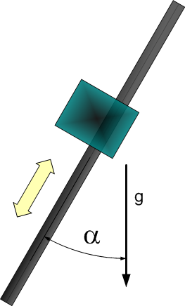
- Tilted axis – an axis with angle α relative to the vertical axis, ranging between 0 and 90 degrees (figure 7). When α = 0 the axis is vertical, and when α = 90 the axis is horizontal (the α parameter is found by the identification (i.e. it is not a user input).
- Vertical axis with a spring.
Rotary axis
The rotary axis type has 3 dynamic model types:
- Simple rotary axis - which its center of mass is located on the rotation axis.
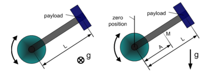
- Horizontal crank-arm axis (figure 8 left).
- Vertical crank-arm axis (figure 8 right).
Example for an identification task that will work for all types mentioned above:
1.  program
2.      dim startPoint as generic joint
3.      dim sineTarget as generic joint
4.      dim SWfreq as generic joint
5.
6.      startPoint = -350
7.      sineTarget = 350
8.      SWfreq = 1.5
9.
10.     with axis
11.         attach
11.	    En = 0
12.	    while En
13.	        sleep 100
14.	    end while
15.	    DynamicModel = 2
16.	    En = 1
17.	    while not En
18.	        sleep 100
19.	    end while
20.
21.	    Move startPoint Abs = 1
22.	    while IsMoving
23.	        sleep 100
24.	    end while
25.
26.	    SineWave sineTarget SineWaveFreq = SWfreq Abs = 1
27.	    sleep 2000
28.	' IdentFilterFreq is a Low pass filter.Frequency should be below 125 Hz
29.	    IdentificationStart IdentFilterFreq = 80
30.	' the time of the identification, you can change time.
31.	    sleep 20000
32.	    IdentificationFinish
33.
34.	    stop
35.	    while IsMoving
36.	        sleep 100
37.	    end while
38.	    proceed
39.	    En = 0
40.
41.	    detach
42.     end with
43. end program
To reuse this code, remember to use frequency and amplitude values that are suited for the application, and also use the suitable dynamic model type.
SCARA robot
The SARA robot has two kinematic models, one with 3 axes (XYZ) and the other with four axes (XYZR).
However, there is only one type of dynamic model which fits both of these kinematics models.
Example for an identification task that will work for 3 axes SCARA:
1.  program
2.      dim startPoint as generic joint
3.      dim sineTarget as generic joint
4.      dim SWfreq as generic joint
5.
6.      startPoint = {-160,-160,0}
7.      sineTarget = {160,160,150}
8.      SWfreq = 0.3*{1,1.27,1.43}
9.
10.     with SCARA
11.         attach
11.	    En = 0
12.	    while En
13.	        sleep 100
14.	    end while
15.	    DynamicModel = 1
16.	    En = 1
17.	    while not En
18.	        sleep 100
19.	    end while
20.
21.	    Move startPoint Abs = 1
22.	    while IsMoving
23.	        sleep 100
24.	    end while
25.
26.	    SineWave sineTarget SineWaveFreq = SWfreq
27.	    sleep 2000
28.	' IdentFilterFreq is a Low pass filter.Frequency should be below 125 Hz
29.	    IdentificationStart IdentFilterFreq = 80
30.	' the time of the identification, you can change time.
31.	    sleep 20000
32.	    IdentificationFinish
33.
34.	    stop
35.	    while IsMoving
36.	        sleep 100
37.	    end while
38.	    proceed
39.	    En = 0
40.
41.	    detach
42.     end with
43. end program
Example for an identification task that will work for 4 axes SCARA:
1.  program
2.      dim startPoint as generic joint
3.      dim sineTarget as generic joint
4.      dim SWfreq as generic joint
5.
6.      startPoint = {-160,-160,0,-350}
7.      sineTarget = {160,160,150,350}
8.      SWfreq = 0.3*{1,1.27,1.43,1.13}
9.
10.     with SCARA
11.         attach
11.	    En = 0
12.	    while En
13.	        sleep 100
14.	    end while
15.	    DynamicModel = 1
16.	    En = 1
17.	    while not En
18.	        sleep 100
19.	    end while
20.
21.	    Move startPoint Abs = 1
22.	    while IsMoving
23.	        sleep 100
24.	    end while
25.
26.	    SineWave sineTarget SineWaveFreq = SWfreq
27.	    sleep 2000
28.	' IdentFilterFreq is a Low pass filter.Frequency should be below 125 Hz
29.	    IdentificationStart IdentFilterFreq = 80
30.	' the time of the identification, you can change time.
31.	    sleep 20000
32.	    IdentificationFinish
33.
34.	    stop
35.	    while IsMoving
36.	        sleep 100
37.	    end while
38.	    proceed
39.	    En = 0
40.
41.	    detach
42.     end with
43. end program
To reuse this code, remember to use frequency and amplitude values that are suited for the application.
Some SCARA robots have coupled joints, usually the 3rd and 4th joints. Currently, the dynamic model of the SCARA robot does not take the coupling into account. Therefore, there may be large errors for coupled joints
DELTA robot
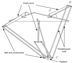
The Delta robot has two kinematic models, one with 3 axes (XYZ) and the other with four axes (XYZR).
However, there is only one type of dynamic model which fits both of these kinematics models.
Example for an identification task that will work for 3 axes Delta:
1.  program
2.      dim startPoint as generic joint
3.      dim sineTarget as generic joint
4.      dim SWfreq as generic joint
5.
6.      startPoint = {-30,-30,-30}
7.      sineTarget = {70,70,70}
8.      SWfreq = 0.3*{1,1.27,1.43}
9.
10.     with DELTA
11.         attach
11.	    En = 0
12.	    while En
13.	        sleep 100
14.	    end while
15.	    DynamicModel = 1
16.	    En = 1
17.	    while not En
18.	        sleep 100
19.	    end while
20.
21.	    Move startPoint Abs = 1
22.	    while IsMoving
23.	        sleep 100
24.	    end while
25.
26.	    SineWave sineTarget SineWaveFreq = SWfreq
27.	    sleep 2000
28.	' IdentFilterFreq is a Low pass filter.Frequency should be below 125 Hz
29.	    IdentificationStart IdentFilterFreq = 80
30.	' the time of the identification, you can change time.
31.	    sleep 20000
32.	    IdentificationFinish
33.
34.	    stop
35.	    while IsMoving
36.	        sleep 100
37.	    end while
38.	    proceed
39.	    En = 0
40.
41.	    detach
42.     end with
43. end program
Example for an identification task that will work for 4 axes Delta:
1.  program
2.      dim startPoint as generic joint
3.      dim sineTarget as generic joint
4.      dim SWfreq as generic joint
5.
6.      startPoint = {-30,-30,-30,-350}
7.      sineTarget = {70,70,70,350}
8.      SWfreq = 0.3*{1,1.27,1.43,1.13}
9.
10.     with DELTA
11.         attach
11.	    En = 0
12.	    while En
13.	        sleep 100
14.	    end while
15.	    DynamicModel = 1
16.	    En = 1
17.	    while not En
18.	        sleep 100
19.	    end while
20.
21.	    Move startPoint Abs = 1
22.	    while IsMoving
23.	        sleep 100
24.	    end while
25.
26.	    SineWave sineTarget SineWaveFreq = SWfreq
27.	    sleep 2000
28.	' IdentFilterFreq is a Low pass filter.Frequency should be below 125 Hz
29.	    IdentificationStart IdentFilterFreq = 80
30.	' the time of the identification, you can change time.
31.	    sleep 20000
32.	    IdentificationFinish
33.
34.	    stop
35.	    while IsMoving
36.	        sleep 100
37.	    end while
38.	    proceed
39.	    En = 0
40.
41.	    detach
42.     end with
43. end program
To reuse this code, remember to use frequency and amplitude values that are suited for the application.
PUMA robot
The PUMA robot has only one kinematic model but it has two different dynamic models.
The first dynamic model is a regular model like the other robots.
The second model is a semi-static model, meaning it will work only for slow movements and static positions. This model takes into account only the gravity and friction forces / torques.
Full regular model
This model identification rules are just like the previous models.
Example for an identification task that will work for PUMA:
1.  program
2.      dim startPoint as generic joint
3.      dim sineTarget as generic joint
4.      dim SWfreq as generic joint
5.
6.      startPoint = {-100,-170,100,-60,-60,-100}
7.      sineTarget = {100,-40,235,60,60,100}
8.      SWfreq = 0.15*{1.56,1,1.31,1.47,1.21,1.17}
9.
10.     with PUMA
11.         attach
11.	    En = 0
12.	    while En
13.	        sleep 100
14.	    end while
15.	    DynamicModel = 1
16.	    En = 1
17.	    while not En
18.	        sleep 100
19.	    end while
20.
21.	    Move startPoint Abs = 1
22.	    while IsMoving
23.	        sleep 100
24.	    end while
25.
26.	    SineWave sineTarget SineWaveFreq = SWfreq
27.	    sleep 2000
28.	' IdentFilterFreq is a Low pass filter.Frequency should be below 125 Hz
29.	    IdentificationStart IdentFilterFreq = 80
30.	' the time of the identification, you can change time.
31.	    sleep 20000
32.	    IdentificationFinish
33.
34.	    stop
35.	    while IsMoving
36.	        sleep 100
37.	    end while
38.	    proceed
39.	    En = 0
40.
41.	    detach
42.     end with
43. end program
To reuse this code, remember to use frequency and amplitude values that are suited for the application.
Semi-static model
The semi-static model identification is a little bit different from all of the examples so far. This model takes into account only gravity and friction forces, in other words it neglects dynamic forces. Therefore, the measurement should include negligible dynamic forces, and this is possible by moving slow.
This identification process is longer than the usual identification progress, it takes approximately 2-3 minutes. In addition, it is advised to perform less than 3 cycles, 1 cycle should be enough.
Also, similar to the previous examples, the semi-static model threshold the velocity of the data points. But unlike the previous examples, here there are two thresholds, one for avoiding very low velocities avoiding numeric errors) and the other for avoiding high velocities (avoiding significant dynamic forces).
Example for such an identification process:
1.  program
2.      dim startPoint as generic joint
3.      dim sineTarget as generic joint
4.      dim SWfreq as generic joint
5.
6.      startPoint = {-100,-170,100,-60,-60,-100}
7.      sineTarget = {100,-40,235,60,60,100}
8.      SWfreq = 0.02*{1.56,1,1.31,1.47,1.21,1.17}
9.
10.     with PUMA
11.         attach
11.	    En = 0
12.	    while En
13.	        sleep 100
14.	    end while
15.	    DynamicModel = 1
16.	    En = 1
17.	    while not En
18.	        sleep 100
19.	    end while
20.
21.	    Move startPoint Abs = 1
22.	    while IsMoving
23.	        sleep 100
24.	    end while
25.
26.	    SineWave sineTarget SineWaveFreq = SWfreq
27.	    sleep 2000
28.	' IdentFilterFreq is a Low pass filter.Frequency should be below 125 Hz
29.	    IdentificationStart IdentFilterFreq = 80
30.	' the time of the identification, you can change time.
31.	    sleep 20000
32.	    IdentificationFinish
33.
34.	    stop
35.	    while IsMoving
36.	        sleep 100
37.	    end while
38.	    proceed
39.	    En = 0
40.
41.	    detach
42.     end with
43. end program
Note the significant low frequencies which cause slow movement.
The Dynamic Models Parameters
This section lists the dynamic parameters for each type of dynamic model.
Rotary Axis
Dynamic Model 1 – simple rotary axis
| Number | Parameter | Comments |
|---|---|---|
| 1 | Total moment of inertia around the rotation axis of the moved part |
- Model equation
Dynamic Model 2 - horizontal crank-arm axis
| Number | Parameter | Comments |
|---|---|---|
| 1 | Total moment of inertia around the rotation axis of the moved part | |
| 2 | Square of length of crank arm (axis to payload) |
- Model equation
Dynamic Model 3 - vertical crank-arm axis
| Number | Parameter | Comments |
|---|---|---|
| 1 | Total moment of inertia around the rotation axis of the moved part | |
| 2 | Square of length of crank arm (axis to payload) | |
| 3 | Mass (without payload) * Gravity * Distance to center of mass | |
| 4 | Gravity * Distance to Payload |
- Model equation
Linear Axis
Dynamic Model 1 - horizontal axis
| Number | Parameter | Comments |
|---|---|---|
| 1 | Total mass of the moved part. |
- Model equation
Dynamic Model 2 - vertical or tilted axis
| Number | Parameter | Comments |
|---|---|---|
| 1 | Total mass of the moved part. | |
| 2 | Constant force due to gravity. | |
| 3 | Gravity coefficient used to consider payload mass. (g = 9.80665) |
- Model equation
SCARA robot
Dynamic Model 1
| Number | Parameter | Comments |
|---|---|---|
| 1 | ||
| 2 | ||
| 3 | ||
| 4 | ||
| 5 | ||
| 6 | ||
| 7 | ||
| 8 |
DELTA robot
Dynamic Model 1
| Number | Parameter | Comments |
|---|---|---|
| 1 | kg*m2 | |
| 2 | kg*m2/sec2 | |
| 3 | kg | |
| 4 | kg*m2 | |
| 5 | kg | |
| 6 | kg | |
| 7 | kg*m2 | |
| 8 | kg*m2 | |
| 9 | m | |
| 10 | m | |
| 11 | ||
| 12 | ||
| 13 | ||
| 14 |
PUMA robot
Dynamic Model 1
Description:
- - Gravity constant
- - Mass of the ith link
- - length of the common normal between the ith and ith+1 joints
- - offset along z axis between the ith and ith+1 joints
- - The distance from the ith joint to the center of mass of the ith link
| Number | Parameter | Comments |
|---|---|---|
| 1 | |
kg/m^2 |
| 2 | kg/m^2 | |
| 3 | kg/m^2 | |
| 4 | kg/m^2 | |
| 5 | kg/m^2 | |
| 6 | kg/m^2 | |
| 7 | kg/m^2 | |
| 8 | kg/m^2 | |
| 9 | kg/m^2 | |
| 10 | kg/m^2 | |
| 11 | kg/m^2 | |
| 12 | kg/m^2 | |
| 13 | kg/m^2 | |
| 14 | kg/m^2 | |
| 15 | kg/m^2 | |
| 16 | kg/m^2 | |
| 17 | kg/m^2 | |
| 18 | kg/m^2 | |
| 19 | kg/m^2 | |
| 20 | kg/m^2 | |
| 21 | kg/m^2 | |
| 22 | kg/m^2 | |
| 23 | kg/m^2 |
Dynamic Model 2 - Gravity
| Number | Parameter | Comments |
|---|---|---|
| 1 | kg*m^2/s^2 | |
| 2 | kg*m^2/s^2 | |
| 3 | kg*m^2/s^2 | |
| 4 | kg*m^2/s^2 |
Identification with a Payload
The IdentificationStart command has a boolean parameter called ‘IdentPayload’. If this parameter is set to false, the identification process is performed regularly. If this parameter is set to true, the identification process identifies only the payload mass or inertia.
In order to identify the payload, one must follow these steps:
- Perform an identification process without the payload.
- Set the dynamic model parameters (by running the identification PRG file).
- Set ‘IdentPayload’ to true and perform an identification process with the payload.
| NOTE | |
| After performing an identification process with the payload and setting ‘IdentPayload’ to true, the identification PRG file will contain the dynamic model parameters form step 1, and the payload parameters from step 3 |
| NOTE | |
| This procedure is valid to all dynamic models except dynamic model 1 of the PUMA robot. |
Explanation of the identification output file
Example of an identification output PRG file. The file is generated at the end of the identification process, and is named: IDNT<group num>.PRG:
1. 'Dynamic parameter identification for PUMA succeeded!
2. 'Identification date and time: 29/03/17 08:17:08
3. 'Max relative torque error: axis 1 = 13.86 %; axis 2 = 8.70 %; axis 3 = 7.79 %; axis 4 = 17.87 %; axis 5 = 23.87 %; axis 6 = 43.85 %; (maximal allowed = 50.00 %)
4. 'Mean relative torque error: axis 1 = 3.18 %; axis 2 = 1.71 %; axis 3 = 1.88 %; axis 4 = 3.59 %; axis 5 = 5.88 %; axis 6 = 12.41 %;
5. 'Signal filter cutoff frequency = 20.000 Hz
6. 'Signal data length = 49876 samples (raw record length = 50000 samples)
7. 'Moving data length: axis 1 = 35998 samples (threshold = 0.038770 rad/s); axis 2 = 35405 samples (threshold = 0.031481 rad/s); axis 3 = 36032 samples (threshold = 0.039294 rad/s); axis 4 = 36785 samples (threshold = 0.041069 rad/s); axis 5 = 34931 samples (threshold = 0.038757 rad/s); axis 6 = 29759 samples (threshold = 0.062830 rad/s);

8.  PROGRAM CONTINUE
9.  ATTACH PUMA

10. PUMA.DynamicParameter[1] = 8.759309007e+01
11. PUMA.DynamicParameter[2] = 1.021832253e+01
12. PUMA.DynamicParameter[3] = 3.042091725e+01
13. PUMA.DynamicParameter[4] = 1.560383089e+00
14. PUMA.DynamicParameter[5] = 0.000000000e+00
15. PUMA.DynamicParameter[6] = 0.000000000e+00

16. A1.ViscousFriction = -1.547427791e+02
17. A1.CoulombFriction = -2.018153298e+01

18. A2.ViscousFriction = -1.603287029e+02
19. A2.CoulombFriction = -4.658045702e+01

20. A3.ViscousFriction = -1.085257604e+02
21. A3.CoulombFriction = -1.961987594e+01

22. A4.ViscousFriction = -1.142833743e+01
23. A4.CoulombFriction = -9.124446870e+00

24. A5.ViscousFriction = -2.468491129e+01
25. A5.CoulombFriction = -3.713111266e+00

26. A6.ViscousFriction = -2.173025205e+00
27. A6.CoulombFriction = -9.724658207e-01

29. PUMA.DynamicModel = 2

30. DETACH PUMA
31. TERMINATE PROGRAM
Line 1-7 give information about the identification process. Line 1 reports if the identification was successful or not.
2. 'Identification date and time: 29/03/17 08:17:08
3. 'Max relative torque error: axis 1 = 13.86 %; axis 2 = 8.70 %; axis 3 = 7.79 %; axis 4 = 17.87 %; axis 5 = 23.87 %; axis 6 = 43.85 %; (maximal allowed = 50.00 %)
Line 2 reports the date and time the identification was made.
Line 3 reports the recorded max relative torque error. The torque error is taken as the TorqueAdditiveCommand (Taddcmd) minus the measured TorqueFeedback. The Taddcmd for this calculation is taken as the Taddcmd that would have been calculated with the identified dynamic parameters as if this movement was performed. In other words, the error is the difference between the real data and the fitted model. The relative torque error is calculated as the torque error divided by the max measured TorqueFeedback (each joint and its max TorqueFeedback value). The max relative torque error, is the maximum value of the relative value for each joint. The formula for the max relative torque error is:
If this value is larger than 50% for one of the joints than the identification is regarded as failed.
4. 'Mean relative torque error: axis 1 = 3.18 %; axis 2 = 1.71 %; axis 3 = 1.88 %; axis 4 = 3.59 %; axis 5 = 5.88 %; axis 6 = 12.41 %;
5. 'Signal filter cutoff frequency = 20.000 Hz
6. 'Signal data length = 49876 samples (raw record length = 50000 samples)
Line 4 reports the mean relative torque error, the mean of the relative torque error over all of the recorded time is taken and displayed for each joint.
Line 5 reports the cutoff frequency that was used for the low pass filter.
Line 6 reports how many data points were recorded.
7. 'Moving data length: axis 1 = 35998 samples (threshold = 0.038770 rad/s); axis 2 = 35405 samples (threshold = 0.031481 rad/s); axis 3 = 36032 samples (threshold = 0.039294 rad/s);
'axis 4 = 36785 samples (threshold = 0.041069 rad/s); axis 5 = 34931 samples (threshold = 0.038757 rad/s); axis 6 = 29759 samples (threshold = 0.062830 rad/s);
Line 7 reports how many data points from each joint were taken for the model fitting. Some data points are discarded if the velocity of the joint in these point is below some threshold (the threshold for each joint is also reported in this line). This is done because the data points with low velocities are causing numerical errors to the model fitting. Therefore, all of the relative errors explained above are calculated only for those points which are taken into account for the model fitting.
10. PUMA.DynamicParameter[1] = 8.759309007e+01
11. PUMA.DynamicParameter[2] = 1.021832253e+01
12. PUMA.DynamicParameter[3] = 3.042091725e+01
13. PUMA.DynamicParameter[4] = 1.560383089e+00
14. PUMA.DynamicParameter[5] = 0.000000000e+00
15. PUMA.DynamicParameter[6] = 0.000000000e+00
Lines 10-15 (for this file) sets the fitted dynamic model parameters.
16. A1.ViscousFriction = -1.547427791e+02
17. A1.CoulombFriction = -2.018153298e+01
18. A2.ViscousFriction = -1.603287029e+02
19. A2.CoulombFriction = -4.658045702e+01
20. A3.ViscousFriction = -1.085257604e+02
21. A3.CoulombFriction = -1.961987594e+01
22. A4.ViscousFriction = -1.142833743e+01
23. A4.CoulombFriction = -9.124446870e+00
24. A5.ViscousFriction = -2.468491129e+01
25. A5.CoulombFriction = -3.713111266e+00
26. A6.ViscousFriction = -2.173025205e+00
27. A6.CoulombFriction = -9.724658207e-01
Lines 16-27 (for this file) sets the fitted friction parameters.
29. PUMA.DynamicModel = 2
Line 29 (for this file) sets the dynamic model that was used for this identification process.
Success condition
The success condition is based on the relative torque error. Each axis should have a max relative torque error value below 50% in order for the identification to be considered as successful.
The torque error is taken as the TorqueAdditiveCommand (Taddcmd) minus the measured TorqueFeedback. The Taddcmd for this calculation is taken as the Taddcmd that would have been calculated with the identified dynamic parameters as if this movement was performed. In other words, the error is the difference between the real data and the fitted model.
The relative torque error is calculated as the torque error divided by the max measured TorqueFeedback (each joint and its max TorqueFeedback value). The max relative torque error, is the maximum value of the relative value for each joint. If this value is larger than 50% for one of the joints than the identification is regarded as failed. Line 4 reports the mean relative torque error, the mean of the relative torque error over all of the recorded time is taken and displayed for each joint. Please note that the relative torque error is evaluated only for the points that stand in a minimum velocity limitation.
The max relative torque error may vary between the different joint. Typically, small joints (with small motors) have larger relative error. This is because the applied torque for these motors is small and the noise in measurement is in the same order of magnitude of the applied torque.
For example: Let’s assume that for a certain point j1.TorqueFeedback = 80 and the j1.TorqueAdditiveCommand = 100. For this point, the j1.TorqueError = 20. Let’s assume that the maximum j1.TorqueFeedback during the recording was 160, then the relative torque error for this point would be: j1.TorqueError/max(j1.TorqueFeedback) = 20/160 = 0.125 = 12.5%
Parameters
Robot models which are supported for dynamic model, have at least one type of dynamic model. These models can be found in the wiki page Dynamic Models. Each model is based on some parameters which are composed of the mass, length and inertia of the different parts of the robot. These are the parameters that are being evaluated with the help of the identification process. The parameters are saved as robot.DynamicParameter[i], where robot is the robot name and i is the number of the parameter as stated in the Dynamic Models page. Each model may have different number of parameters.
After the dynamic parameter, appear the viscous friction and coulomb friction parameters: axis.ViscousFriction, axis.CoulombFriction . Each joint of the robot has these two parameters which define its friction coefficients.
In addition to these parameters, the user should consider to set the maximum allowed value for the additive torque command. This could be set with the property TorqueThreshold, e.g. a1.TorqueThreshold = 200. If the Taddcmd exceeds this value, than the softMC reports an error.
Including the identification output file in setup
In order for the dynamic model to take effect you should simply run the IDNT<group num>.PRG file while the robot is disabled (en = 0). Note that this should come after the robot setup. In order to automatically load the dynamic model configuration during the system initialization and robot setup, simply add the line:
Load IDNT<group num>.PRG To the end of your AUTOEXEC.PRG or STARTPRG.PRG file, after the robot setup.
Explanation of the identification process recording file
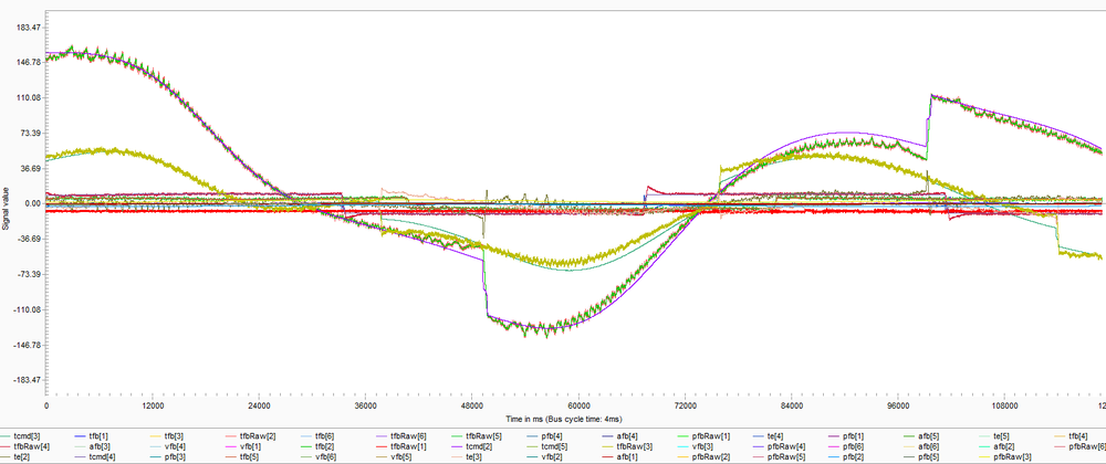
Another file that is generated at the end of the identification process is the data recording file. This file is named: IDNT<group num>.REC. This file contains all of the relevant data that was used by the identification process. Here are the parameters which are displayed for each joint:
- tfbRaw – The raw recorded data of the TorqueFeedback (tfb) property.
- pfbRaw – The raw recorded data of the PositionFeedback (pfb) property.
- tfb – The filtered recorded data of the TorqueFeedback (tfb) property.
- pfb – The filtered recorded data of the PositionFeedback (pfb) property.
- vfb – The filtered recorded data of the VelocityFeedback (vfb) property.
- afb – The filtered recorded data of the AccelerationFeedback (afb) property.
- tcmd – The torque command generated by the fitted model. The found dynamic parameters and the collected data are used to calculate this property. In regular mode, this property will actually be TorqueAdditiveCommand (Taddcmd).
- te – The TorqueError (te) calculated by the difference of the tcmd and tfb data.
This file can be used for better debugging and troubleshooting, as well as for better understanding the identification process. At figure 15 you can find example of an identification output REC file:
Demonstration of tracking improvements (settling, position error)
SCARA Robot
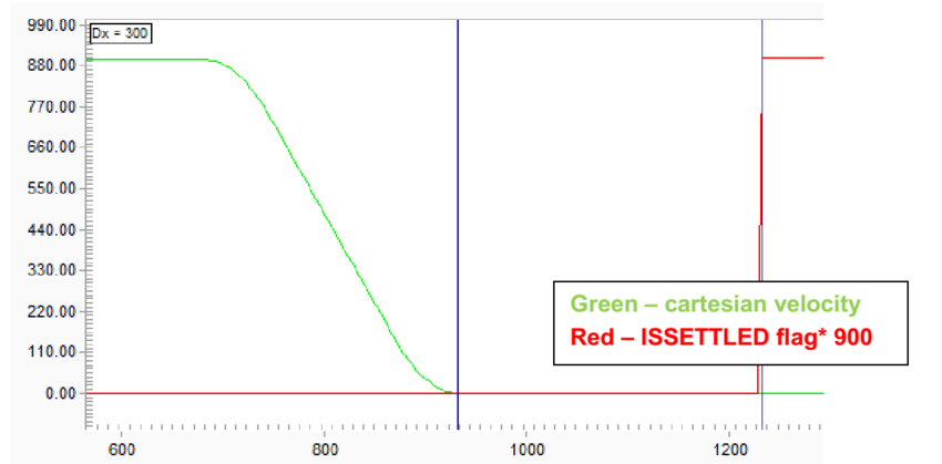
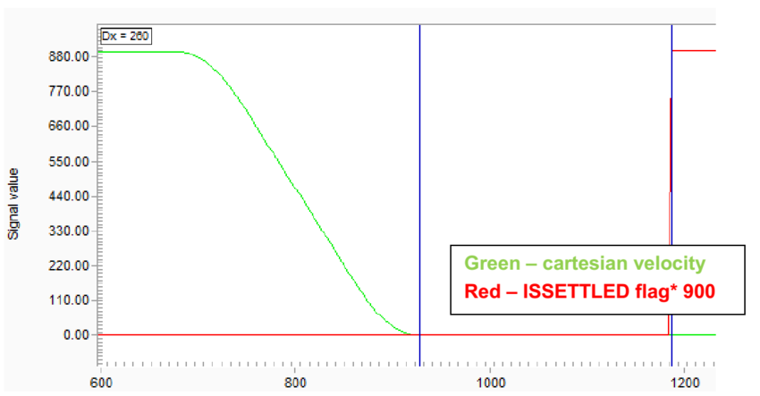
An experiment was made for a 4 axes scara robot with and without dynamic model. The robot was commanded to move 600[mm] in a straight line with linear velocity of 900[mm/s]. The cartesian velocity of the robot and the ISSETTLED property were recorded during this motion (figure 16 and 17, the ISSETTLED property is scaled by 3000).
The ISSETTLED property indicates whether the actual element position is within the specified settling range. The settling range is defined by the PESETTLE property and is further qualified by the TIMESETTLE property. When the motion profiler has completed, the absolute value of the position error (Target Position – Actual Position) is compared to the PESETTLE property. When the result is less than or equal to this property for the time given by TIMESETTLE, the ISSETTLED flag is set. For this example, the PESETTLE was taken as 0.001.
Therefore, one could expect that a shorter settling time indicates on better performance.
Figures 16 and 17 display the recorded data from the experiment. The results are that the settling time for this motion without dynamic model is 300 ms, and the settling time with dynamic model is 260 ms – ~86.7% of the original settling time.
DELTA Robot
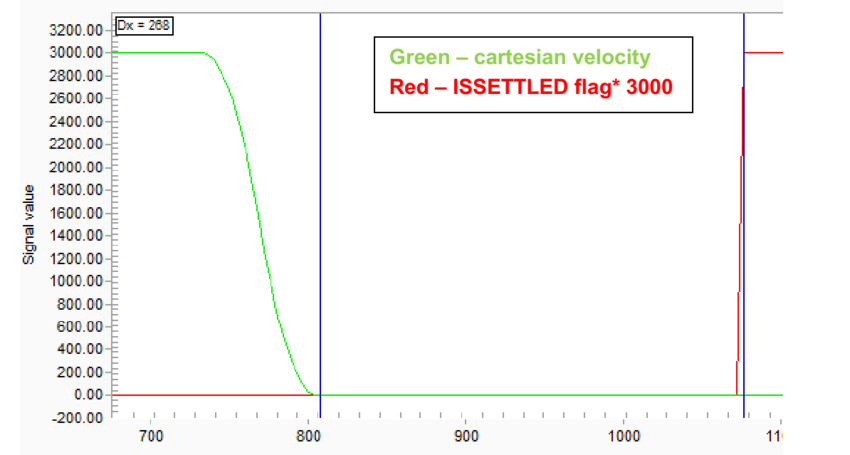
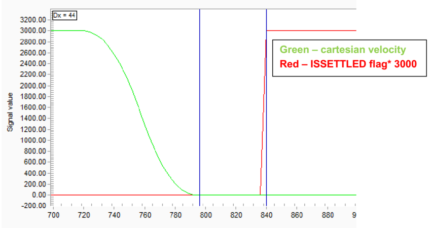
An experiment was made for a 3 axes delta robot with and without dynamic model. The robot was commanded to move 550[mm] in a straight line with linear velocity of 3000[mm/s]. The cartesian velocity of the robot and the ISSETTLED property were recorded during this motion (figure 17 and 18, the ISSETTLED property is scaled by 3000).
The ISSETTLED property indicates whether the actual element position is within the specified settling range. The settling range is defined by the PESETTLE property and is further qualified by the TIMESETTLE property. When the motion profiler has completed, the absolute value of the position error (Target Position – Actual Position) is compared to the PESETTLE property. When the result is less than or equal to this property for the time given by TIMESETTLE, the ISSETTLED flag is set. For this example, the PESETTLE was taken as 0.05.
Therefore, one could expect that a shorter settling time indicates on better performance.
Figures 17 and 18 display the recorded data from the experiment. The results are that the settling time for this motion without dynamic model is 268 ms, and the settling time with dynamic model is 44 ms – ~16.5% of the original settling time.
PUMA Robot
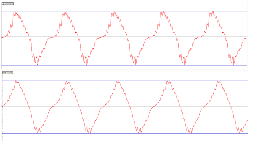
An experiment was made with and without dynamic model. Axis 3 was commanded to oscillate with the SineWave command while axis 2 was commanded to stay at 0.
Figure 19 shows axis 2 position error for the cases with (top) and without (bottom) dynamic model. The peak to peak amplitude for the cases with and without dynamic model are ~0.6e-3 and ~1e-3 correspondingly. It means that using the dynamic model reduced ~40% of the error for this example.
Collision detection
The dynamic model allows to enable a more delicate collision detection feature. Without the dynamic model, the softMC can detect a collision by thresholding the position error of the robot or joints. However, when using the dynamic model of the robot, a collision can be detected by thresholding the torque error. The torque error reacts quicker than the position error, hence enabling a more delicate collision detection.
In order to activate the thresholding over the torque error for a certain joint, set the property TorqueErrorEnable (Teen) to 1, e.g. a1.Teen = 1. One more property to set is the TorqueErrorMax (Temax), e.g. a1.Temax = 10. This property set the maximum allowed torque error which above it softMC reports an error. Note that the Temax property may vary between joints, usually the bigger the joint’s motor the bigger Temax that the user should allow. Also note that as the dynamic model identification results get more accurate, the Temax can be decreased as the torque error gets smaller.
One last property to consider is the TorqueErrorFilter property. If the torque feedback is noisy, the Temax value can be exceed due to noise which causes false collision triggering. Filtering this noise helps to achieve better collision detection procedure. This property gets values in the range of 0.0 to 1.0. The filter is a very simple averaging filter, it performs as follows:
when TE is the TorqueError property, and TEF is the TorqueErrorFilter property.
Note that usually the largest error occurs in the beginning, ending or direction changing of the movement. Therefore, the magnitude of the errors in these cases determine what the Temax value will be. Nevertheless, these cases are also characterized with very low velocities. Hence, it is possible to write an application that monitors the torque error and joint velocities, and ignore the cases when the velocity is small, or perhaps increase the Temax just for these cases. As a result, the collision detection feature can become very sensitive
Review of the possible reasons for an identification failure
This section reviews some possible reasons that may cause poor results or a failure of the identification process. The next section reviews how to identify these reasons.
Movement is too slow
The dynamic identification model requires that the robot joints will move in a high velocity, as mentioned in section 3. When the joints move at a low velocity, the developed torque in the joints opposes mainly the joints friction and gravity torques, and the acceleration and inertia terms are relatively small. Therefore, the dynamic model parameters identification will perform poorly. Furthermore, the identification process ignores data that is under certain minimal velocity, so moving slowly can also cause for lack of data.
That being said, in such a case, the output PRG identification file may report that the identification process was successful and the resulting max relative errors can be small. However, later, when attempting to move at higher velocities than the velocities used during the identification process, the additive torque command predictions will most likely perform poorly.
Figure 20 shows an example for an identification output REC file for a 3 axes delta robot where the motion was slow during the identification. It is noticeable that the data is very noisy. The reason for that is that the movement is slow, hence the developed torques are small and the relative noise is large
Figure 21 shows the torque error for the same delta robot and the same motion. The top figure is the result of the motion using the retrieved parameters from a slow identification process and the bottom figure is the result of the motion using the retrieved parameters from a good identification process. One can see that the torque errors increase dramatically for the case with slow identification process
Movement is too fast
This problem is less likely to happen, but still, it can cause poor results or a failure of the identification process.
If the robot joints are brought to their limits, the motor torque can reach to a saturation value. The current dynamic model does not take saturation into account, therefore, if saturation occurred, it will cause poor identification results
Movement duration is too short
The identification is based on the collected data that is recorded during the robot movement. If there is not enough data, the identification may overfit the data and will predict accurately just for the region of the collected data. In such case the identification may be reported as successful, hence the user has to judge if the collected data is sufficient. A rule of thumb is that each joint should complete at least 3 cycles.
Movement region is too small
The identification is based on the collected data that is recorded during the robot movement. If the data is not scattered over the entire work area of the robot, the identification may overfit the data and will predict accurately just for the region of the collected data.
In such case the identification may be reported as successful, hence the user has to judge if the collected data is sufficient. A rule of thumb is that each joint should reach position values closely to its negative and positive position limits.
TorqueFactor properties are not configured well
The dynamic model of each robot is based on the MKS system of units defines, hence the torque feedback values should be in units of [Nm]. If the TorqueFactor properties are not configured well than the torque feedback will not have suitable values and the model equations will be wrong.
In such a case, the identification process will perform poorly and the identified model parameters will not be correct.
Wrong type of DynamicModel property
Some kinematic models are assigned with more than one type of dynamic model. These different models are in order to deal with different configurations. For example, a linear axis may be horizontal, vertical, or tilted in a certain angle, each of those configurations has a different dynamic model and different DynamicModel property value.
If a wrong DynamicModel value is set, the identification process will perform poorly.
How to assess what is the failure reason based on the output files
This section reviews some possible failure results of the generated identification files and the identification process. The failures may be the failure of the identification process, or successful identification process with poor performance results.
Identification process failure
An identification failure is the case where one of the joints results with a max relative error larger than 50%. Here are some reasons that may cause this result:
- One or more of the joints moved too slow. This can be identified in the output PRG file in lines 6 and 7. Line 6 reports how many data points were collected for each joint. Line 7 reports how many points are with a velocity larger than the velocity threshold. If the data points number after thresholding for one or more of the joints is significantly smaller than the total number of collected points, then it means that this joint moved too slow.
- One or more of the joints reached saturation. This can be identified in the output REC file. Open the output REC file and observe only the following properties of the joint in subject: tfb, tcmd and te. Saturation can be identified by seeing that the tfb reaches a sudden plateau while the tdcmd continues regularly.
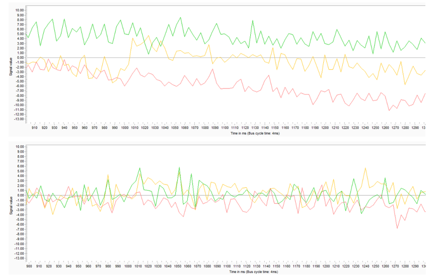
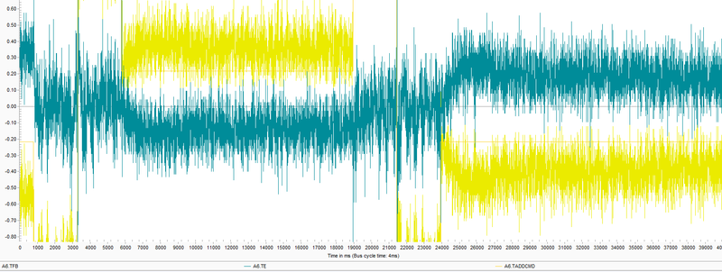
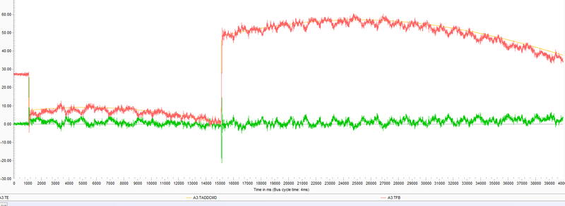
- Large noise for small joints. For some systems, the noise can be in the same order of magnitude of the mean operation currents. In such cases, the relative torque error may be very big although the net torque error is small. In such cases it is recommended to use the resultant dynamic parameters as received in the output PRG file even though the identification failed (taking into account that there aren’t any more problems). In order to indicate that this is the problem, open the output REC file and observe only the following properties of the joint in subject: tfb, tcmd and te. Then it is possible to observe if the large error occurs due to noise. Figure 22 shows an example of noise in the same order of magnitude of the mean operation currents and figure 23 shows an example of relative small noise magnitude
Identification process success but poor real time prediction results
An identification process can be reported as successful but perform poorly in real time. For some reason, the model was able to fit the data well enough, but the model is not good enough for other movements during regular operation. This usually happens because the robot did not cover major parts of its working space during identification process. Here are some reasons that may cause this result:
- The amplitude of one or more of the joints is not big enough and does not cover the range of movement of the joint. This could be viewed in the output REC file, or simply rechecking that the commanded amplitude is large enough.
- The identification process duration was too short (relative to the joints velocity). It can be identified by looking at the output REC file. Look at each joint’s pfb property. If one or more of the joints doesn’t complete at least 3 cycles, increasing the identification duration time (or the joints velocity) should help.
- The chosen frequencies are overlapping or don’t allow enough diversity of locations. It can be identified by looking at the output REC file. Look at all joints pfb properties together. If two or more joints seems to oscillate together, or overlap after small amount of cycles, or oscillate very similarly, try to change the frequencies of the problematic joints.
Test specifications
This section describes how to test the dynamic model feature and check that it works properly. The test procedures are comprised of recording specific properties while performing some kind of a robot motion. The minimum required properties to record are Tfb, Taddcmd, Te. Testing can be divided into two types: one is checking that the torques predictions accuracy is reasonably small for all types of movements; and the other is checking that the robot performance (e.g. settling time, vibration, etc.) improves with the dynamic model activated.
Testing the accuracy is equivalent to testing the torque error. In order to test the torque error, simply generate a task that generates some variation of movements and record the required properties while it’s running. Alternatively, if the robot application task is already known, one can use this task in order to perform this testing. Simply run the task while recording the Tfb, Taddcmd and Te properties. Then, observe the recording (especially Te property) and decide if the achieved accuracy if satisfactory or not.

